SICP 2.19: Counting Change Revisited

From SICP section 2.2.1 Representing Sequences

Exercise 2.19 asks us to modify the change counting procedure from section 1.2.2 (which we looked at in depth in exercise 1.14). We need to modify the program so that it takes a list of coins to be used instead of having the denominations hard coded as they were originally. The following lists of coins are provided:

(define us-coins (list 50 25 10 5 1))
(define uk-coins (list 100 50 20 10 5 2 1 0.5))

We're also provided with the following modified version of the cc procedure:

(define (cc amount coin-values)
  (cond ((= amount 0) 1)
        ((or (< amount 0) (no-more? coin-values)) 0)
        (else
         (+ (cc amount
                (except-first-denomination coin-values))
            (cc (- amount
                   (first-denomination coin-values))
                coin-values)))))

All that's left for us to do is define the procedures first-denomination, except-first-denomination, and no-more? in terms of primitive list operations. These procedures are very straightforward.

; return true if passed an empty list
(define (no-more? coin-values)
  (if (null? coin-values) true false))

; return all coin values except the first
(define (except-first-denomination coin-values)
  (cdr coin-values))

; return only the first coin value
(define (first-denomination coin-values)
  (car coin-values))

> (cc 100 us-coins)
292
> (cc 100 uk-coins)
104561

Finally, we're asked if the order of the list coin-values affects the answer produced by cc. We can find out quickly enough by experiment.

; reversed list of us coins
(define su-coins (list 1 5 10 25 50))

> (cc 100 us-coins)
292
> (cc 100 su-coins)
292

We can see that the order doesn't matter. This is because the procedure recursively evaluates every sub-list after subtracting the value of the first coin from the target amount. It doesn't matter if that value is the smallest, largest, or even if the values are shuffled.


Related:

For links to all of the SICP lecture notes and exercises that I've done so far, see The SICP Challenge.

SICP 2.18: Reversing a List

From SICP section 2.2.1 Representing Sequences

Exercise 2.18 asks us to define a procedure reverse that takes a list as its argument and returns a list with the same elements in reverse order.

We'll be using the append procedure given in the text which takes two lists and appends the second list to the end of the first:

(define (append list1 list2)
   (if (null? list1)
       list2
       (cons (car list1) (append (cdr list1) list2))))

We can reverse a list by appending the car of the list to the reverse of the cdr of the list. (See how easy it is to start thinking in Scheme?) In other words, we just move the first item to the end of the list after reversing the remaining items. This means reverse will make a recursive call to itself, so we also need a base case to make the recursion stop. We can just stop when we reach an empty list.

(define (reverse items)
 (if (null? items)
     items
     (append (reverse (cdr items)) (list (car items)))))

Once again, we can test it out with a few example lists from the text.

> (reverse (list 1 2 3 4))
(4 3 2 1)
> (reverse (list 1 4 9 16 25))
(25 16 9 4 1)
> (reverse (list 1 3 5 7))
(7 5 3 1)
> (reverse (list 23 72 149 34))
(34 149 72 23)

Related:

For links to all of the SICP lecture notes and exercises that I've done so far, see The SICP Challenge.

SICP 2.17: Last Item in a List

From SICP section 2.2.1 Representing Sequences

Exercise 2.17 asks us to define a procedure last-pair that returns a list that contains only the last element of a given (non-empty) list.

Earlier in SICP section 2.2.1 we saw that a list is represented in Scheme as a chain of pairs.


Our new procedure needs to return a list, so we need to be careful not to simply return the last value in the list, or even the last pair.

There are several correct ways to do this, but here's a recursive solution (based on the length example from the text) that uses the method of "cdring down" the list.

(define (last-pair items)
  (if (null? (cdr items))
      (list (car items))
      (last-pair (cdr items))))

The first line checks to see if the cdr of the list of items passed in is nil. If it is, the second line creates a new list from the car of the items. If not, the last line makes a recursive call to last-pair with the remaining items in the list.

We can verify that it works by testing it with several of the example lists from the chapter.

> (last-pair (list 1 2 3 4))
(4)
> (last-pair (list 1 4 9 16 25))
(25)
> (last-pair (list 1 3 5 7))
(7)
> (last-pair (list 23 72 149 34))
(34)

Related:

For links to all of the SICP lecture notes and exercises that I've done so far, see The SICP Challenge.

SICP 2.12 - 2.16: Extended Exercise: Interval Arithmetic (Part 2)

From SICP section 2.1.4 Extended Exercise: Interval Arithmetic

The solutions in the first half of this extended exercise, SICP 2.7 - 2.11: Extended Exercise: Interval Arithmetic (Part 1), are only one possible way to approach the problem of implementing interval arithmetic. Another way to represent intervals is as a center value and an added tolerance. The following alternate constructor and selectors are supplied in the text:

; Represent intervals as a center value and a width
(define (make-center-width c w)
   (make-interval (- c w) (+ c w)))

(define (center i)
   (/ (+ (lower-bound i) (upper-bound i)) 2))

(define (width i)
   (/ (- (upper-bound i) (lower-bound i)) 2))

Here's a test case to show how it works:

> (define a (make-center-width 5 1))
> a
(4 . 6)
> (center a)
5
> (width a)
1

A third way of representing intervals, often used by engineers, is as a center value and a percent tolerance measured as the ratio of the width of the interval to its center value.



Exercise 2.12 asks us to define a constructor make-center-percent that takes a center and a percent tolerance and creates the desired interval. We'll also need to define a selector percent that extracts the percentage tolerance for a given interval.

We can define our new constructor in terms of make-center-width. We'll make our procedure take a whole number percentage p.

(define (make-center-percent c p)
   (make-center-width c (* c (/ p 100.0))))

Since the percent tolerance of an interval is the ratio of the interval's width to its center, we can implement percent in terms of the provided width and center procedures.

(define (percent i)
   (* 100.0 (/ (width i) (center i))))

Here's how we'd define the same interval as before with the new constructor:

> (define a (make-center-percent 5 20))
> a
(4.0 . 6.0)
> (center a)
5.0
> (width a)
1.0
> (percent a)
20.0

Exercise 2.13 asks us to show that there is, for small tolerances, a simple formula for the approximate percentage tolerance of the product of two intervals in terms of the tolerances of the factors. We can assume that all numbers are positive.

Recall the old definition of interval multiplication that we used was:

[a,b] × [c,d] = [min (ac, ad, bc, bd), max (ac, ad, bc, bd)]

Since we're assuming all positive numbers for this exercise, we can change the definition to a simpler form:

[a,b] × [c,d] = [ac, bd]

Now we need to complicate things again and look at what it means to represent an interval in terms of its center (c_i) and percent tolerance (p_i).

i = [c_i - c_i(p_i/100), c_i + c_i(p_i/100)]
i = [c_i(1 - p_i/100), c_i(1 + p_i/100)]

Multiplying two intervals x and y together would be:

xy = [c_xc_y(1 - p_x/100)(1 - p_y/100), c_xc_y(1 + p_x/100)(1 + p_y/100)]

We can use the FOIL method to combine some of the terms above.

(1 - p_x/100)(1 - p_y/100) = (1 - p_y/100 - p_x/100 + p_xp_y/10,000)

= 1 - (p_x + p_y)/100 + p_xp_y/10,000

(1 + p_x/100)(1 + p_y/100) = 1 + p_y/100 + p_x/100 + p_xp_y/10,000
= 1 + (p_x + p_y)/100 + p_xp_y/10,000

Inserting those back into the interval notation we get:

xy = [c_xc_y(1 - (p_x + p_y)/100 + p_xp_y/10,000), c_xc_y(1 + (p_x + p_y)/100 + p_xp_y/10,000)]

Since the exercise lets us assume that both p_x and p_y are small, and because we're only looking for an approximation, we can ignore the p_xp_y/10,000 terms because they'll be very small.

xy = [c_xc_y(1 - (p_x + p_y)/100), c_xc_y(1 + (p_x + p_y)/100)]

Now we have things back in terms of an interval's center and percent tolerance. The center of the product of the two intervals is c_xc_y, and the percent tolerance is (p_x + p_y). The approximate percentage tolerance of the product of the two intervals is the sum of the tolerances of the two factors.

We can check this with a quick example.

> (define a (make-center-percent 5 2))
> (define b (make-center-percent 10 3))
> (define c (mul-interval a b))
> (percent c)
4.997001798920647

Electrical resistor values are often expressed as a center value and a percent tolerance, so an engineer writing programs that work with resistances would be likely to make use of an interval arithmetic library. The formula for parallel resistors can be written in two algebraically equivalent ways:

and
The following two programs implement the two different computations:

(define (par1 r1 r2)
   (div-interval (mul-interval r1 r2)
                 (add-interval r1 r2)))

(define (par2 r1 r2)
   (let ((one (make-interval 1 1)))
      (div-interval one
                    (add-interval (div-interval one r1)
                                  (div-interval one r2)))))

Exercise 2.14 asks us to demonstrate that the two programs above give different answers for the same inputs by investigating the behavior of the system on a variety of arithmetic expressions.

First we'll make some intervals and look at the results of interval division in terms of center and percent.

> (define a (make-center-percent 100 5))
> (define b (make-center-percent 200 2))
> (define aa (div-interval a a))
> aa
(0.9047619047619049 . 1.1052631578947367)
> (define ab (div-interval a b))
> ab
(0.46568627450980393 . 0.5357142857142857)
> (center aa)
1.0050125313283207
> (center ab)
0.5007002801120448
> (percent aa)
9.97506234413964
> (percent ab)
6.993006993006991

What's notable here is that the center of the result of dividing an interval by itself is not 1, but just an approximation to it. This will be important when we explain what's wrong with our interval system in the next exercise. For now we're just trying to show that something isn't right.

We can use the same intervals that we defined above to illustrate the difference between the two parallel resistance procedures.

> (define apb1 (par1 a b))
> (define apb2 (par2 a b))
> apb1
(60.25889967637541 . 73.6082474226804)
> apb2
(63.986254295532646 . 69.32038834951456)

> (define apa1 (par1 a a))
> (define apa2 (par2 a a))
> apa1
(42.97619047619048 . 58.026315789473685)
> apa2
(47.5 . 52.49999999999999)

This verifies that there is a significant difference between the two procedures.


Exercise 2.15 points out that a formula to compute with intervals using the library we've been developing will produce tighter error bounds if it can be written in such a form that no variable that represents an uncertain number (an interval) is repeated. The conclusion is that par2 is a "better" program for parallel resistances than par1. We need to explain if this is correct, and why.

First, this is a good time to show that the two formulas used to develop par1 and par2 are algebraically equivalent. We're trying to show that


We'll start with the formula on the right hand side and derive the formula on the left. To do so, all we really need to do is multiply by R₁/R₁ and R₂/R₂. Since both of these fractions equal 1, these are valid transformations.


So the formulas are algebraically equivalent, but they don't give the same answer. Why could that be? The answer lies in the trick we used just now to show equivalence. We used the ratios R₁/R₁ and R₂/R₂ to change the formula and said that it was okay because that's just like multiplying by 1. But R₁ and R₂ represent resistor values, which are intervals, and we saw in exercise 2.14 that dividing an interval by itself doesn't equal 1, it just approximates it. Transforming the equation in this way introduces error. That's why the observation that we can get tighter error bounds if we avoid repeating variables that represent uncertain numbers is correct.



Exercise 2.16 asks us to explain why equivalent algebraic expressions may lead to different answers. It goes on to ask if we can devise an interval-arithmetic package that does not have this shortcoming, or if the task is impossible.

As the text points out, this is a very difficult problem. Wikipedia to the rescue.

The so-called dependency problem is a major obstacle to the application of interval arithmetic. Although interval methods can determine the range of elementary arithmetic operations and functions very accurately, this is not always true with more complicated functions. If an interval occurs several times in a calculation using parameters, and each occurrence is taken independently then this can lead to an unwanted expansion of the resulting intervals.

...

In general, it can be shown that the exact range of values can be achieved, if each variable appears only once. However, not every function can be rewritten this way.

In short, no we cannot design an interval arithmetic package that does not have this shortcoming in the general case. The best we can do, as was indicated in the previous exercise, is to try and write formulas that avoid repeating variables that represent intervals. This is not always possible.


Related:

For links to all of the SICP lecture notes and exercises that I've done so far, see The SICP Challenge.

SICP 2.7 - 2.11: Extended Exercise: Interval Arithmetic (Part 1)

From SICP section 2.1.4 Extended Exercise: Interval Arithmetic

Section 2.1.4 is a small project that has us design and implement a system for working with intervals (objects that represent the range of possible values of an inexact quantity). We need to implement interval arithmetic as a set of arithmetic operations for combining intervals. The result of adding, subtracting, multiplying, or dividing two intervals is itself an interval, representing the range of the result. We're provided with the procedures for adding, multiplying, and dividing two intervals.

The minimum value the sum could be is the sum of the two lower bounds and the maximum value it could be is the sum of the two upper bounds:

(define (add-interval x y)
   (make-interval (+ (lower-bound x) (lower-bound y))
                  (+ (upper-bound x) (upper-bound y))))

The product of two intervals is computed by finding the minimum and the maximum of the products of the bounds and using them as the bounds of the resulting interval.

(define (mul-interval x y)
   (let ((p1 (* (lower-bound x) (lower-bound y)))
         (p2 (* (lower-bound x) (upper-bound y)))
         (p3 (* (upper-bound x) (lower-bound y)))
         (p4 (* (upper-bound x) (upper-bound y))))
     (make-interval (min p1 p2 p3 p4)
                    (max p1 p2 p3 p4))))

We can divide two intervals in terms of the mul-interval procedure by multiplying the first interval by the reciprocal of the second. Note that the bounds of the reciprocal interval are the reciprocal of the upper bound and the reciprocal of the lower bound, in that order.

(define (div-interval x y)
   (mul-interval x
                 (make-interval (/ 1.0 (upper-bound y))
                                (/ 1.0 (lower-bound y)))))

Exercise 2.7 gives us the implementation for make-interval and asks us to complete the interval abstraction by implementing the selectors.

; by convention the bounds are added in lower-upper order
(define (make-interval a b) (cons a b))

(define (upper-bound intrvl)
   (cdr intrvl))

(define (lower-bound intrvl)
   (car intrvl))

Now that we have most of our definitions in place, we can start testing some of the given procedures.

> (define a (make-interval 5 10))
> (define b (make-interval 10 20))
> (add-interval a b)
(15 . 30)
> (mul-interval a b)
(50 . 200)
> (div-interval a b)
(0.25 . 1.0)

Exercise 2.8 asks us to implement a procedure for computing the difference of two intervals, sub-interval, using reasoning similar to that used to implement add-interval. The smallest value possible when subtracting interval y from interval x is to subtract the upper bound of y from the lower bound of x. The largest result of subtracting interval y from interval x is to subtract the lower bound of y from the upper bound of x.

; interval subtraction: [a,b] − [c,d] = [a − d, b − c]
(define (sub-interval x y)
   (make-interval (- (lower-bound x) (upper-bound y))
                  (- (upper-bound x) (lower-bound y))))

We can test this with a few different intervals to show that it works whether the intervals overlap or not.

> (define a (make-interval 1 10))
> (define b (make-interval 50 100))
> (define c (make-interval 5 20))
> (sub-interval b a)
(40 . 99)
> (sub-interval a b)
(-99 . -40)
> (sub-interval a c)
(-19 . 5)
> (sub-interval c a)
(-5 . 19)

Exercise 2.9 defines the width of an interval as half the difference between its upper and lower bounds. For some arithmetic operations the width of the result of combining two intervals is a function only of the widths of the argument intervals, whereas for others the width of the combination is not a function of the widths of the argument intervals. We are to show that the width of the sum (or difference) of two intervals is a function only of the widths of the intervals being added (or subtracted).

I think this is best proven mathematically by showing that the width of the sum of two intervals is the same as the sum of the widths of two intervals. We start with a couple of definitions for interval addition and computing the width of an interval:

[a,b] + [c,d] = [a + c, b + d]
width([x, y]) = (y - x) / 2

Now we can combine these to come up with a formula for the width of the sum of two intervals.

width([a, b] + [c, d]) = width([a + c, b + d])
= ((b + d) - (a + c)) / 2

Finally, we can derive a formula for the sum of the widths of two intervals.

width([a, b]) + width([c, d]) = (b - a) / 2 + (d - c) / 2
= ((b - a) + (d - c)) / 2
= ((b + d) - (a + c)) / 2

This is the same formula we derived above. This proves that if we add any two intervals with widths x and y, the width of the resulting interval will always be z, no matter what the bounds of the intervals are.

To prove that this is not the case for interval multiplication we can use a simple counterexample.

> (define a (make-interval 2 4))
> (define b (make-interval 5 10))
> (define c (make-interval 10 15))
> (mul-interval a b)
(10 . 40)
> (mul-interval a c)
(20 . 60)

The intervals b and c have the same width, but when we multiply each of them by interval a, the resulting intervals have different widths. This means that the width of the product of two intervals cannot be a function of only the widths of the operands.


Exercise 2.10 points out that it is not clear what it means to divide by an interval that spans zero. We need to modify the provided div-interval routine to check for this condition and signal an error if it occurs.

Before we make the required modifications, let's take a closer look at the div-interval procedure to see what the problem is.

(define (div-interval x y)
   (mul-interval x
                 (make-interval (/ 1.0 (upper-bound y))
                                (/ 1.0 (lower-bound y)))))

If the interval y spans zero, then there's a small problem with this portion of the code:

(make-interval (/ 1.0 (upper-bound y))
              (/ 1.0 (lower-bound y))

If y is the interval [-10, 10], for example, then the snippet above would produce the interval [0.1, -0.1], which has a lower bound that is higher than its upper bound.

To fix the problem we can just do as the exercise suggests and signal an error if a zero-spanning interval is found in the divisor.

; Exercise 2.10
(define (spans-zero? y)
   (and (<= (lower-bound y) 0)
        (>= (upper-bound y) 0)))

(define (div-interval x y)
   (if (spans-zero? y)
       (error "Error: The denominator should not span 0.")
       (mul-interval x
                 (make-interval (/ 1.0 (upper-bound y))
                                (/ 1.0 (lower-bound y))))))

Run an example in your interpreter to verify.

> (define a (make-interval 2 5))
> (define b (make-interval -2 2))
> (div-interval a b)
. . Error: The denominator should not span 0.

Exercise 2.11 suggests that by testing the signs of the endpoints of the intervals, we can break mul-interval into nine cases, only one of which requires more than two multiplications. We are to rewrite mul-interval using this suggestion.

The suggestion is based on the result of multiplication of two numbers with the same or opposite signs. For each interval there are three possibilities, both signs are positive, both are negative, or the signs are opposite. (Note that an interval with the signs [+, -] is not allowed, since the lower bound would be higher than the upper bound.) Since there are two intervals to check, that makes nine possibilities. All nine possibilities are listed below.

[+, +] * [+, +]
[+, +] * [-, +]
[+, +] * [-, -]

[-, +] * [+, +]
[-, +] * [-, +]
[-, +] * [-, -]

[-, -] * [+, +]
[-, -] * [-, +]
[-, -] * [-, -]

For most of the combinations above, we can see directly which pairs need to be multiplied to form the resulting interval. For example, if all values are positive, then multiplying the two upper bounds and two lower bounds are the only two products we need to find. The only case where we need to do more than two multiplications is in the case [-, +] * [-, +], since the product of the two lower bounds could possibly be larger than the product of the two upper bounds.

Note that the following code is much less readable and would be harder to maintain than the original procedure. In addition to that, without benchmarking both procedures we aren't even sure which one is faster. The trade-off in maintainability certainly doesn't seem to be worth any potential savings you might get from eliminating two multiplications from most cases. The developer who suggested this enhancement should probably have their commit access revoked (and be shot out of a cannon).

; Exercise 2.11
(define (mul-interval x y)
   (let ((xlo (lower-bound x))
         (xhi (upper-bound x))
         (ylo (lower-bound y))
         (yhi (upper-bound y)))
   (cond ((and (>= xlo 0)
               (>= xhi 0)
               (>= ylo 0)
               (>= yhi 0))
          ; [+, +] * [+, +]
          (make-interval (* xlo ylo) (* xhi yhi)))
         ((and (>= xlo 0)
               (>= xhi 0)
               (<= ylo 0)
               (>= yhi 0))
          ; [+, +] * [-, +]
          (make-interval (* xhi ylo) (* xhi yhi)))
         ((and (>= xlo 0)
               (>= xhi 0)
               (<= ylo 0)
               (<= yhi 0))
          ; [+, +] * [-, -]
          (make-interval (* xhi ylo) (* xlo yhi)))
         ((and (<= xlo 0)
               (>= xhi 0)
               (>= ylo 0)
               (>= yhi 0))
          ; [-, +] * [+, +]
          (make-interval (* xlo yhi) (* xhi yhi)))
         ((and (<= xlo 0)
               (>= xhi 0)
               (<= ylo 0)
               (>= yhi 0))
          ; [-, +] * [-, +]
          (make-interval (min (* xhi ylo) (* xlo yhi))
                         (max (* xlo ylo) (* xhi yhi))))
         ((and (<= xlo 0)
               (>= xhi 0)
               (<= ylo 0)
               (<= yhi 0))
          ; [-, +] * [-, -]
          (make-interval (* xhi ylo) (* xlo ylo)))
         ((and (<= xlo 0)
               (<= xhi 0)
               (>= ylo 0)
               (>= yhi 0))
          ; [-, -] * [+, +]
          (make-interval (* xlo yhi) (* xhi ylo)))
         ((and (<= xlo 0)
               (<= xhi 0)
               (<= ylo 0)
               (>= yhi 0))
          ; [-, -] * [-, +]
          (make-interval (* xlo yhi) (* xlo ylo)))
         ((and (<= xlo 0)
               (<= xhi 0)
               (<= ylo 0)
               (<= yhi 0))
          ; [-, -] * [-, -]
          (make-interval (* xhi yhi) (* xlo ylo))))))

We'll need several test cases to make sure we get good coverage of all possible conditions.

> (define a (make-interval 2 4))
> (define b (make-interval -2 4))
> (define c (make-interval -4 -2))
> (mul-interval a a)
(4 . 16)
> (mul-interval a b)
(-8 . 16)
> (mul-interval a c)
(-16 . -4)
> (mul-interval b a)
(-8 . 16)
> (mul-interval b b)
(-8 . 16)
> (mul-interval b c)
(-16 . 8)
> (mul-interval c a)
(-16 . -4)
> (mul-interval c b)
(-16 . 8)
> (mul-interval c c)
(4 . 16)

Related:

For links to all of the SICP lecture notes and exercises that I've done so far, see The SICP Challenge.

SICP 2.6: Church numerals

From SICP section 2.1.3 What Is Meant by Data?

Exercise 2.6 introduces us to the idea that in a language that can manipulate procedures, we can get by without integers altogether. The implementation of 0 and the operation of adding 1 are given as

(define zero (lambda (f) (lambda (x) x)))

(define (add-1 n)
   (lambda (f) (lambda (x) (f ((n f) x)))))

This representation is known as Church numerals, after its inventor, Alonzo Church, the logician who invented the λ calculus.

It's important to note that the definition for zero above does not evaluate to the integer 0, it is just a representation for 0.

> zero
#<procedure:zero>

A Church numeral is a procedure that takes one argument, and that argument is itself another procedure that also takes one argument. The procedure zero represents the integer 0 by returning a procedure that applies its input procedure zero times. The Church numeral one should return a procedure that applies its input procedure once, two should return a procedure that applies its input procedure twice, and so on. This is how Church numerals represent integers, by applying their input procedure the exact number of times that the numerals are supposed to represent.

Our job in this exercise is to define one and two directly (not in terms of zero and add-1). We'll do that by using substitution to evaluate (add-1 zero) to see what the resulting procedural definition should be. We also need to give a direct definition for addition of two Church numerals (not in terms of repeated application of add-1).

Before we begin, we'll need some method for testing Church numerals to make sure they do what we expect them to do. We'll need a simple procedure to pass to each Church numeral as an argument so that we can see it gets evaluated the correct number of times. The inc procedure should do nicely. (You can replace inc with any procedure you like, just make it one that's easy to mentally calculate several repetitions of.)

(define (inc n)
   (+ n 1))

We can use inc to show that zero does not call its input parameter, or more precisely, it calls its input procedure zero times.

> ((zero inc) 0)
0
> ((zero inc) 1)
1
> ((zero inc) 2)
2

Now let's define one and two in the way that the book warns us not to, just to make sure they behave as we expect. I'll give the assigned implementations later.

> (define one (add-1 zero))
> (define two (add-1 one))
> ((one inc) 0)
1
> ((one inc) 1)
2
> ((two inc) 0)
2
> ((two inc) 1)
3

So we can see that the procedure returned by one applies inc one time, and the procedure returned by two applies it twice. Now let's use substitution to evaluate (add-1 zero), giving us the direct definition of the Church numeral one.

(add-1 zero)

; retrieve the body of add-1 and substitute zero for its parameter n
(lambda (f) (lambda (x) (f ((zero f) x))))

; retrieve the body of zero and substitute
(lambda (f) (lambda (x) (f ((lambda (x) x) x))))

; simplify
(lambda (f) (lambda (x) (f x)))

So we can define one directly as:

(define one
   (lambda (f) (lambda (x) (f x))))

Next we can define two by evaluating (add-1 one) using exactly the same principles.

(add-1 one)

; retrieve the body of add-1 and substitute one for its parameter n
(lambda (f) (lambda (x) (f ((one f) x))))

; retrieve the body of one and substitute
(lambda (f) (lambda (x) (f ((lambda (x) (f x)) x))))

; simplify
(lambda (f) (lambda (x) (f (f x))))

So two is defined directly as:

(define two
   (lambda (f) (lambda (x) (f (f x)))))

Just as was explained earlier, the Church numeral one takes a procedure as an argument and returns a procedure that applies the input procedure once. The only difference in the Church numeral two is that it applies its input procedure twice.

Add these definitions in the Scheme interpreter and test them out the same as before.

> ((one inc) 0)
1
> ((one inc) 5)
6
> ((two inc) 3)
5
> ((two inc) 7)
9

Now we need to figure out how to add two Church numerals. We can see from the definition of add-1 that all it does is takes a Church numeral, n, and wraps one additional function call around it.

(define (add-1 n)
   (lambda (f) (lambda (x) (f ((n f) x)))))

We can implement Church numeral addition by using the same approach. We'll take two Church numerals m and n. Instead of wrapping n in one extra function call, we'll wrap it in m extra calls.

(define (add-church m n)
   (lambda (f) (lambda (x) ((m f) ((n f) x)))))

We can now use add-church to define several more Church numerals for testing.

> (define three (add-church one two))
> (define four (add-church two two))
> (define seven (add-church three four))
> ((three inc) 0)
3
> ((four inc) 0)
4
> ((seven inc) 0)
7

Related:

For links to all of the SICP lecture notes and exercises that I've done so far, see The SICP Challenge.

SICP 2.5: Representing Pairs as a Product

From SICP section 2.1.3 What Is Meant by Data?

Exercise 2.5 asks us to show that we can represent pairs of non-negative integers using only numbers and arithmetic operations if we represent the pair a and b as the integer that is the product 2^a3^b. We're to give the corresponding definitions of the procedures cons, car, and cdr.

This exercise reminds me of the old adage that just because you can do something doesn't mean that you should. The implementations of cons, car, and cdr that follow are severely limited in that they can only join pairs of integers, not pairs of any type of data as we've seen before.

Regardless, here is what is meant by representing non-negative integers as the product 2^a3^b. Note that because 2 and 3 are both prime, and due to the fundamental theorem of arithmetic, any integer values that we insert for a and b will result in a unique value for the product 2^a3^b. Because the product is unique, we're able to get back the original values of a and b by just storing the product and remembering the rule we used to generate it.

The definition of cons is straightforward from the requirements using the built-in Scheme expt procedure.

(define (cons a b)
  (* (expt 2 a)
     (expt 3 b)))

But once we've combined two integers in this way, how do we separate them again? For example, if we evaluate (cons 5 6) we get a result of 23328. The corresponding implementation of car needs to take the value 23328 and tell us what that the original value of a was 5. We can do that by counting the number of times 23328 is evenly divisible by 2. Since 2 and 3 have no factors in common, once you divide all the 2s out of 23328 you'll be left with a power of 3. Since we're going to be doing the same thing for cdr, we'll define a general procedure that can be reused.

There's no easy way to find out how many times one number evenly divides another other than simply trying to divide by the number in a loop and testing for a remainder. If there was a quick formula that we could apply to get the answer in one step then prime factorization would be much easier than it is. We'll have to use an iterator to do this in as few steps as possible.

; count the number of times n is evenly divisible by d
(define (num-divs n d)
  (define (iter x result)
    (if (= 0 (remainder x d))
        (iter (/ x d) (+ 1 result))
        result))
  (iter n 0))

I tested this with the example values above to make sure it gives the correct results.

> (num-divs 23328 2)
5
> (num-divs 23328 3)
6

Now we can define both car and cdr in terms of num-divs.

(define (car x)
  (num-divs x 2))

(define (cdr x)
  (num-divs x 3))

Finally, we can use the axiom of pairs (from Lecture 2B) to show that our new definitions for cons, car, and cdr work together as they should.

> (car (cons 4 7))
4
> (cdr (cons 4 7))
7

Related:

For links to all of the SICP lecture notes and exercises that I've done so far, see The SICP Challenge.

SICP 2.4: Implementing cons, car, and cdr

From SICP section 2.1.3 What Is Meant by Data?

Exercise 2.4 gives us the following alternative procedual implementation for creating pairs.

(define (cons x y)
  (lambda (m) (m x y)))

(define (car z)
  (z (lambda (p q) p)))

Using this implementation, we are told to verify that (car (cons x y)) yields x for any objects x and y using the substitution model from section 1.1.5.

Once we've done that, we need to write the corresponding definition of cdr.

Our first step to verifying that this implementation for cons and car work should be to put the code in a Scheme interpreter and see them work.

> (car (cons 2 3))
2
> (car (cons 15 "Hello"))
15
> (car (cons "Hi!" 42))
"Hi!"

Now let's use the substitution model to show that the following always yields x

(car (cons x y))

First we retrieve the body of cons

(lambda (m) (m x y))

We could replace the formal parameters x and y with the arguments 2 and 3 (or any others that we choose) at this point, but I'm going to keep working with x and y. Let's substitute the body of cons.

(car (lambda (m) (m x y)))

Now we can retrieve the body of car and substitute it.

((z (lambda (p q) p)) (lambda (m) (m x y)))

The car procedure takes a procedure z as an argument and applies it to (lambda (p q) p), so there's one more substitution we need to do here before this step is really done. We need to take the second lambda in the expression above and replace z with it.

((lambda (m) (m x y)) (lambda (p q) p))

That might look scary, but it's just a procedure applied to another procedure. Since the procedure on the left takes one formal parameter, we can substitute the procedure on the right for that parameter.

((lambda (p q) p) x y)

Now it should be clear that this expression is a procedure that takes two parameters p and q, and passes two parameters to it. The procedure returns the first of the two parameters passed to it, so this expression simplifies to x.

The definition for cdr that corresponds to the above implementation of car is simply

(define (cdr z)
  (z (lambda (p q) q)))

We can test it out the same way we originally tested the code provided in the text,
by running it in the interpreter.

>  (cdr (cons 2 3))
3
> (cdr (cons 15 "Hello"))
"Hello"
> (cdr (cons "Hi!" 42))
42

Related:

For links to all of the SICP lecture notes and exercises that I've done so far, see The SICP Challenge.

SICP 2.3: Rectangles in a plane

From SICP section 2.1.2 Abstraction Barriers

Exercise 2.3 asks us to build on the results of exercise 2.2 and implement a representation for rectangles in a plane. In addition to a constructor and selectors for a representation of a rectangle, we'll also need to implement procedures for computing the perimeter and area of a given rectangle. Once we've done that we'll need to implement a different representation for rectangles. The challenge is to design a system with suitable abstraction barriers so that the area and perimeter procedures will work with either rectangle representation.

First let's look at a few different ways to represent rectangles. To simplify things, we'll assume that the sides of the rectangle are to be perpendicular to the x- and y-axes of the coordinate plane.

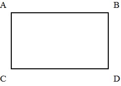
The most obvious representation would be to combine four points (ignoring the fact that four points might not form a rectangle and just accepting any four points for this representation). We could easily implement this representation since we already have a representation for points in a plane.


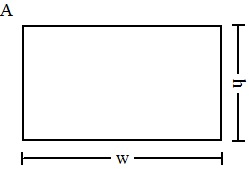
Next, we could represent a rectangle as a single point along with a width and a height. This would make it very easy to calculate the perimeter and area of a given rectangle.


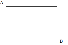
Another representation could be to store two opposite corners of the rectangle. This would give us just enough information to calculate the width and the height, from which we can calculate the perimeter and area.


You can probably think of several other representations such as storing all four segments that make up the sides of a rectangle, storing only two adjacent sides, or storing the segment that joins two opposite corners forming a diagonal. These would all work, but some require us to store more information than we really need.

The first implementation will be the third one pictured above where a rectangle is represented by two opposite corners. The constructor will simply join two points together. The selctors will return the width and height of the rectangle. The width and height are calculated by taking the absolute value of the difference between the x- and y-coordinates respectively.

; rectangle constructor
; join two opposite corners
(define (make-rect a b) (cons a b))

; rectangle selectors
(define (rect-width r)
   (abs (- (x-point (car r)) (x-point (cdr r)))))

(define (rect-height r)
   (abs (- (y-point (car r)) (y-point (cdr r)))))

With that done, we can implement procedures for computing the perimeter and area of a rectangle.

(define (rect-perimeter r)
   (* 2 (+ (rect-width r) (rect-height r))))

(define (rect-area r)
   (* (rect-width r) (rect-height r)))

We can test it out by defining two points, creating a rectangle, and displaying its perimeter and area.

> (define a (make-point 0 0))
> (define b (make-point 2 10))
> (define r (make-rect a b))
> (display (rect-perimeter r))
24
> (display (rect-area r))
20

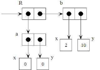
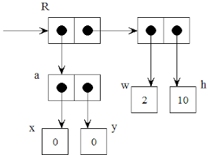
The box-and-pointer diagram of the rectangle created above shows how the individual elements are stored. The rectangle itself is made up of two points (from the last exercise), each of which are themselves made up of an x and a y value. The rect-width and rect-height selectors are used to access these x and y values to calculate the width and height of the rectangle.


Now we can implement an alternate representation of a rectangle and show that we can use the same procedures for perimeter and area. The easiest will be the second pictured above, where we represent a rectangle by a single point and its width and height.

; rectangle constructor
; combine a point, a width, and a height
(define (make-rect a w h) (cons a (cons w h)))

; rectangle selectors
(define (rect-width r)
   (car (cdr r)))

(define (rect-height r)
   (cdr (cdr r)))

Using the new constructor and selectors we can test that the old rect-perimeter and rect-area procedures work unchanged.

> (define a (make-point 0 0))
> (define r (make-rect a 2 10))
> (display (rect-perimeter r))
24
> (display (rect-area r))
20

The box-and-pointer diagram of this rectangle reveals that the elements are laid out exactly the same way internally, but the rectangle is different conceptually.



This time the rectangle is made up of a point, a width, and a height. The corresponding rect-width and rect-height procedures access their values directly rather than computing them.


Related:

For links to all of the SICP lecture notes and exercises that I've done so far, see The SICP Challenge.

SICP 2.2: Line segments in a plane

From SICP section 2.1.2 Abstraction Barriers

Exercise 2.2 asks us to define a constructor and selectors for creating line segments in a plane. A line segment is represented by a starting point and an ending point. We'll also need to create a constructor and selectors for creating points in a plane, where a point is represented by an x and a y value. Finally, using these constructors and selectors we need to define a midpoint-segment procedure that takes a line segment as its argument and returns the midpoint of that segment. A procedure for printing points is provided.

(define (print-point p)
   (newline)
   (display "(")
   (display (x-point p))
   (display ",")
   (display (y-point p))
   (display ")"))

If you watched lecture 2B on compound data, you already know that the procedures for defining points in a plane are going to be very similar to the original procedures for defining rational numbers. All we need to do to construct a point is glue its two parts together.

; point constructor
(define (make-point x y) (cons x y))

; point selectors
(define (x-point p) (car p))
(define (y-point p) (cdr p))

The procedures for defining segments are almost the same, only the names will change.

; segment constructor
(define (make-segment a b) (cons a b))

; segment selectors
(define (start-segment s) (car s))
(define (end-segment s) (cdr s))

Remember that we're just gluing two "things" together. It only matters conceptually (which is pretty important, really) that the two things in this case are points, while before they were primitive numbers. The mechanism for combining them is the same.

Next we need to use the midpoint formula to define a procedure for computing the midpoint of a segment. The midpoint is defined as the average of the x-values and the y-values of the two endpoints of the segment.



Our new procedure needs to take a segment and return a point.

(define (midpoint-segment s)
    (make-point (/ (+ (x-point (start-segment s))
                     (x-point (end-segment s)))
                  2)
               (/ (+ (y-point (start-segment s))
                    (y-point (end-segment s)))
                  2)))

There are a few examples illustrating the midpoint formula on Purplemath. I'll use those to test with.

Find the midpoint between (–1, 2) and (3, –6).
Answer: P = (1, -2)

> (define a (make-point -1 2))
> (define b (make-point 3 -6))
> (define s (make-segment a b))
> (define m (midpoint-segment s))
> (print-point m)

(1,-2)

Find the midpoint between (6.4, 3) and (–10.7, 4).
Answer: P = (–2.15, 3.5)

> (define a (make-point 6.4 3))
> (define b (make-point -10.7 4))
> (define s (make-segment a b))
> (define m (midpoint-segment s))
> (print-point m)

(-2.1499999999999995,7/2)

Related:

For links to all of the SICP lecture notes and exercises that I've done so far, see The SICP Challenge.

SICP 2.1: Rational numbers

From SICP section 2.1.1 Example: Arithmetic Operations for Rational Numbers

Exercise 2.1 asks us to define a better version of make-rat that handles both positive and negative arguments. Here's the last version from the text, along with several example cases to show how it works:

(define (make-rat n d)
  (let ((g (gcd n d)))
    (cons (/ n g) (/ d g))))

> (define x (make-rat 1 2))
> (print-rat x)

1/2
> (define x (make-rat -1 -2))
> (print-rat x)

-1/-2
> (define x (make-rat 1 -2))
> (print-rat x)

1/-2
> (define x (make-rat -1 2))
> (print-rat x)

-1/2

The new version of make-rat should normalize the sign so that if the resulting rational number is positive, both the numerator and denominator are positive. If the rational number is negative, only the numerator should be negative.

We can correct make-rat by checking to see if the denominator is negative. If it is, we need to multiply both the numerator and denominator by -1 to normalize the result. If not, we just pass the arguments bare to cons.

(define (make-rat n d)
  (let ((g (gcd n d)))
    (if (< d 0)
        (cons (/ (* n -1) g) (/ (* d -1) g))
        (cons (/ n g) (/ d g)))))

We can use the same definitions as before to see the results from the new make-rat procedure.

> (define x (make-rat 1 2))
> (print-rat x)

1/2
> (define x (make-rat -1 -2))
> (print-rat x)

1/2
> (define x (make-rat 1 -2))
> (print-rat x)

-1/2
> (define x (make-rat -1 2))
> (print-rat x)

-1/2

Related:

For links to all of the SICP lecture notes and exercises that I've done so far, see The SICP Challenge.

SICP Lecture 2B: Compound Data

Structure and Interpretation of Computer Programs
Compound Data
Covers Text Section 2.1: Introduction to Data Abstraction

You can download the video lecture or stream it on MIT's OpenCourseWare site. It's also available on YouTube.

This lecture is presented by Professor Harold Abelson

Chapter 1 of SICP was all about procedures using primitive data, and how to build higher and higher abstractions using procedures. The next chapter will be all about combining primitive data into compound data abstractions.

The fundamental means of combining primitive data in Scheme is to glue two things together into a pair. We use the cons function to combine two things together to make a pair. Once you've combined them you need something to get the two separate parts back. To do that you use the car and cdr functions.

(cons x y) - constructs a pair whose first part is x and second part is y.

(car p) - selects the first part of the pair p.

(cdr p) - selects the second part of the pair p.

The convention for drawing diagrams of pairs is called box-and-pointer notation.




The formal way of describing the behavior of cons, car, and cdr, and how they interact with one another is called the axiom for pairs:

For any x and y:
(car (cons x y)) is x
(cdr (cons x y)) is y

Representing rational numbers

The text defines a system for representing rational numbers using pairs.

(define (make-rat n d) (cons n d))

(define (numer x) (car x))
(define (denom x) (cdr x))

These functions are called a constructor (make-rat) and selectors (numer and denom). Once we have the simple data abstraction in place, we can use the abstraction to define other procedures that work with rational numbers using the rules of rational number arithmetic.

(define (add-rat x y)
   (make-rat (+ (* (numer x) (denom y))
                (* (numer y) (denom x)))
             (* (denom x) (denom y))))

(define (sub-rat x y)
   (make-rat (- (* (numer x) (denom y))
                (* (numer y) (denom x)))
             (* (denom x) (denom y))))

(define (mul-rat x y)
   (make-rat (* (numer x) (numer y))
             (* (denom x) (denom y))))

(define (div-rat x y)
   (make-rat (* (numer x) (denom y))
             (* (denom x) (numer y))))

(define (print-rat x)
   (newline)
   (display (numer x))
   (display "/")
   (display (denom x)))

Data abstraction separates the use of a data object from its representation. You could define add-rat and the other procedures without using data abstraction by directly using cons, car, and cdr. The point of isolating the use from the representation is that you have to capture the idea of a conceptual entity.


Compound Data

Like procedure definition, the real power of compound data is that we can use it to create building blocks that can themselves be used to create more complex data structures. Using the same method we used for creating rational numbers, we could also create a set of functions for representing points in a plane. From those points we can build line segments, from line segments we can build two-dimensional shapes. We could keep going and build as many abstractions on top of each other as we need to represent any system we want.

Closure - the means of combination in the system are such that when you put things together with them you can then put those things together using the same means. The system is closed. (This use of the word "closure" is in the same sense as it's used in abstract algebra. The Lisp community also uses the same word for an unrelated concept.)

Once you can combine two things, the closure property allows you to combine as many things as you want.



We'll see later in the text that this is how lists are formed in Scheme.


What are pairs really?

The last section of the lecture shows that pairs can be build out of nothing at all. If Scheme didn't have primitive functions cons, car, and cdr we could define them ourselves.

(define (cons a b)
  (lambda (pick)
     (cond ((= pick 1) a)
           ((= pick 2) b))))

(define (car x) (x 1))
(define (cdr x) (x 2))

In this implementation cons returns a procedure, not a pair. The definitions for car and cdr take the procedure supplied by cons and apply it to 1 and 2 respectively. If this system satisfies the axiom for pairs that we saw earlier, then it's a perfectly reasonable implementation. In the lecture, mechanical substitution is used to prove that this system does satisfy the axiom for pairs.


Related:

For links to all of the SICP lecture notes and exercises that I've done so far, see The SICP Challenge.

Kaprekar's constant

Kaprekar's constant is arrived at by following these steps:

1. Take any four-digit number whose digits are not all the same (leading zeroes are allowed).
2. Sort the digits in descending then ascending order, making the largest and smallest possible 4-digit numbers composed of those digits. (Add leading zeroes if necessary.)
3. Subtract the smaller number from the larger number. The result will be another 4-digit number.
4. Repeat the process starting with the result.

For example, starting with the digits 0827 (today's date) we get:

8720 - 0278 = 8442
8442 - 2448 = 5994
9954 - 4599 = 5355
5553 - 3555 = 1998
9981 - 1899 = 8082
8820 - 0288 = 8532
8532 - 2358 = 6174

If we continue the process outlined above the result will always be 6174.

7641 - 1467 = 6174

The amazing thing is that starting with any 4-digit number whose digits are not all the same will result in 6174 in at most seven steps. 6174 is called the Kaprekar constant for 4-digit numbers after Dattaraya Ramchandra Kaprekar who discovered the property in 1949.

There's a Kaprekar constant for 3-digit numbers as well. Following the same procedure above starting with any 3-digit number whose digits are not all the same will end in the result of 495 in at most six steps. Applying the same process to base 10 numbers with any other number of digits will result in either zero or a cycle that never ends. (Check out the article Mysterious number 6174 by Yutaka Nishiyama for the proof.)

You can see the results of the Kaprekar routine for 3-digit or 4-digit numbers using the utility below. Just enter a number in the first field and click the "Calculate" button. The results will appear below.

SICP 1.46: Iterative improvement

From SICP section 1.3.4 Procedures as Returned Values

Exercise 1.46 asks us to combine several of the concepts we've learned throughout the first chapter of SICP into a procedure that generalizes the iterative improvement strategy. Iterative improvement is the process where we start with an initial guess, test if the guess is good enough, then improve the guess and start the process over again with the new guess. Our iterative-improve procedure will take two procedures as arguments and return a procedure as its value. The first argument will define a method for telling whether a guess is good enough, and the second will define a method for improving a guess. The returned procedure will take a guess as its argument and will keep improving that guess until it is good enough. Finally, we will rewrite the sqrt procedure from section 1.1.7 and the fixed-point procedure from section 1.3.3 using iterative-improve.

A good starting point is to take a look at the original versions of the two procedures mentioned in the exercise and see what they have in common.

; sqrt procedure and sub-procedures from SICP 1.1.7
(define (sqrt x)
   (sqrt-iter 1.0 x))

(define (sqrt-iter guess x)
   (if (good-enough? guess x)
       guess
       (sqrt-iter (improve guess x)
                  x)))

(define (improve guess x)
   (average guess (/ x guess)))

(define (average x y)
   (/ (+ x y) 2))

(define (good-enough? guess x)
 (< (abs (- (square guess) x)) 0.001))

(define (square x) (* x x))


; fixed-point procedure from SICP 1.3.3
(define tolerance 0.00001)
(define (fixed-point f first-guess)
   (define (close-enough? v1 v2)
     (< (abs (- v1 v2)) tolerance))
   (define (try guess)
     (let ((next (f guess)))
       (if (close-enough? guess next)
           next
           (try next))))
   (try first-guess))

Besides the similarities that you might expect from the description in the exercise, these two procedures also both make use of helper functions to perform the required iteration, sqrt-iter and try. We'll need a helper function in iterative-improve as well, and this will be the function that will be returned by the procedure. (We can't use a lambda to define the returned procedure like past exercises in this section because the returned procedure in this case needs to call itself recursively. To do that, it needs a name.)

(define (iterative-improve good-enough? improve)
   (define (iter-imp guess)
     (if (good-enough? guess)
         guess
         (iter-imp (improve guess))))
   iter-imp)

The solution doesn't require a lot of explanation. We define the procedure iter-imp that takes a guess as its only parameter. If the guess is good enough (as judged by the function passed in as the first argument to iterative-improve) we just return the guess. If not, we call iter-imp again with a new guess that we get by calling the improve function that was passed in as the second parameter to iterative-improve.

Let's see how we can redefine sqrt in terms of iterative-improve.

(define (sqrt x)
   ((iterative-improve (lambda (guess)
                         (< (abs (- (square guess) x))
                            0.001))
                       (lambda (guess)
                         (average guess (/ x guess))))
   1.0))

Here I've taken the implementation of the procedures for good-enough? and improve almost exactly from the earlier sqrt solution, but I've recast them as lambdas. Since iterative-improve returns a procedure, we give it an initial guess of 1.0 to start things off. This implementation of sqrt works much the same as the original.

> (sqrt 4)
2.0000000929222947
> (sqrt 16)
4.000000636692939
> (sqrt 100)
10.000000000139897
> (sqrt 1000)
31.622782450701045

The reimplementation of fixed-point is very similar.

(define (fixed-point f first-guess)
   ((iterative-improve (lambda (guess)
                         (< (abs (- (f guess) guess))
                            0.00001))
                       (lambda (guess)
                         (f guess)))
    first-guess))

The good-enough? procedures for sqrt and fixed-point are nearly identical. The improve procedure for fixed-point is simpler though, because to improve a guess when finding a fixed point, you just apply the function whose fixed point you're trying to find to the guess.

To test the new fixed-point procedure, we can use the procedure we defined in exercise 1.35 to approximate the golden ratio.

> (fixed-point (lambda (x) (+ 1 (/ 1 x))) 2.0)
1.6180371352785146

Related:

For links to all of the SICP lecture notes and exercises that I've done so far, see The SICP Challenge.