SICP 2.56 - 2.58: Symbolic Differentiation

From SICP section 2.3.2  Example: Symbolic Differentiation

This section of SICP presents an application of symbol manipulation in the form of the following procedure that performs symbolic differentiation of algebraic expressions.

(define (deriv exp var)
  (cond ((number? exp) 0)
        ((variable? exp)
         (if (same-variable? exp var) 1 0))
        ((sum? exp)
         (make-sum (deriv (addend exp) var)
                   (deriv (augend exp) var)))
        ((product? exp)
         (make-sum
           (make-product (multiplier exp)
                         (deriv (multiplicand exp) var))
           (make-product (deriv (multiplier exp) var)
                         (multiplicand exp))))
        (else
         (error "unknown expression type -- DERIV" exp))))

The following supporting procedures are required by deriv. Each one is explained in the text.

(define (variable? x) (symbol? x))

(define (same-variable? v1 v2)
  (and (variable? v1) (variable? v2) (eq? v1 v2)))

(define (make-sum a1 a2) (list '+ a1 a2))
(define (make-product m1 m2) (list '* m1 m2))

(define (sum? x)
  (and (pair? x) (eq? (car x) '+)))

(define (addend s) (cadr s))
(define (augend s) (caddr s))

(define (product? x)
  (and (pair? x) (eq? (car x) '*)))

(define (multiplier p) (cadr p))
(define (multiplicand p) (caddr p))

With these definitions, we can perform differentiation on algebraic expressions in Scheme's familiar prefix notation.

> (deriv '(+ x 3) 'x)
(+ 1 0)
> (deriv '(* x y) 'x)
(+ (* x 0) (* 1 y))
> (deriv '(* (* x y) (+ x 3)) 'x)
(+ (* (* x y) (+ 1 0)) (* (+ (* x 0) (* 1 y)) (+ x 3)))

This procedure returns results that are correct, but the expressions are not in their simplest form. For example, instead of (+ 1 0) we'd like the procedure to simplify the expression to 1. Similarly, the expression (+ (* x 0) (* 1 y)) can be simplified to y. We only need to change the constructors make-sum and make-product to simplify the resulting expressions. We can change make-sum so that if both its arguments are numbers, make-sum will return their sum. Also, if either of the arguments is 0, then make-sum will return the other summand (whether it's a number or a symbol).

(define (make-sum a1 a2)
  (cond ((=number? a1 0) a2)
        ((=number? a2 0) a1)
        ((and (number? a1) (number? a2)) (+ a1 a2))
        (else (list '+ a1 a2))))

Similarly, make-product should return 0 if either of its arguments is 0, and if either of its arguments is 1 it should return the other argument.

(define (make-product m1 m2)
  (cond ((or (=number? m1 0) (=number? m2 0)) 0)
        ((=number? m1 1) m2)
        ((=number? m2 1) m1)
        ((and (number? m1) (number? m2)) (* m1 m2))
        (else (list '* m1 m2))))

Both of these new implementations make use of the =number? procedure to check whether an expression is equal to an expected value.

(define (=number? exp num)
  (and (number? exp) (= exp num)))

Here's how the improved procedures work with the same three examples.

> (deriv '(+ x 3) 'x)
1
> (deriv '(* x y) 'x)
y
> (deriv '(* (* x y) (+ x 3)) 'x)
(+ (* x y) (* y (+ x 3)))

The first two resulting expressions are now in simplest form. The third is greatly improved, but could still be better.

Exercise 2.56 asks us to extend the deriv procedure to handle more kinds of expressions. We're to implement the differentiation rule

 $\frac{d(u^n)}{dx} = nu^{(n-1)} (\frac{du}{dx})$ 

by adding a new clause to the deriv program and defining appropriate procedures exponentiation?, base, exponent, and make-exponentiation. (We'll use the symbol ** to denote exponentiation.) We'll also build in the rules that anything raised to the power 0 is 1 and any expression raised to the power 1 is the expression itself. We can base the implementations of exponentiation?, base, and exponent on the corresponding procedures used for sums and products.

(define (exponentiation? x)
  (and (pair? x) (eq? (car x) '**)))

(define (base e) (cadr e))
(define (exponent e) (caddr e))

Similarly, our implementation of make-exponentiation will be based on the updated versions of make-sum and make-product, since we're going to build in two rules of exponentiation that will simplify resulting expressions.

(define (make-exponentiation base exponent)
  (cond ((=number? exponent 0) 1)
        ((=number? exponent 1) base)
        ((and (number? base) (number? exponent)) (expt base exponent))
        (else (list '** base exponent))))

The last step before testing is to extend the deriv procedure itself to recognize and handle exponentiation.

(define (deriv exp var)
  (cond ((number? exp) 0)
        ((variable? exp)
         (if (same-variable? exp var) 1 0))
        ((sum? exp)
         (make-sum (deriv (addend exp) var)
                   (deriv (augend exp) var)))
        ((product? exp)
         (make-sum
           (make-product (multiplier exp)
                         (deriv (multiplicand exp) var))
           (make-product (deriv (multiplier exp) var)
                         (multiplicand exp))))
        ((exponentiation? exp)
         (make-product
          (make-product (exponent exp)
                        (make-exponentiation
                         (base exp)
                         (make-sum (exponent exp) -1)))
          (deriv (base exp) var)))
        (else
         (error "unknown expression type -- DERIV" exp))))

We can test the extended implementation of deriv using an example from the beginning of the current section of the text. "For example, if the arguments to the procedure are $ax^2 + bx + c$ and x, the procedure should return $2ax + b$." I'll translate the expression to prefix notation in multiple steps so we can see the effect that each term has on the result.

> (deriv '(** x 2) 'x)
(* 2 x)
> (deriv '(* a (** x 2)) 'x)
(* a (* 2 x))
> (deriv '(+ (* a (** x 2)) (* b x)) 'x)
(+ (* a (* 2 x)) b)
> (deriv '(+ (+ (* a (** x 2)) (* b x)) c) 'x)
(+ (* a (* 2 x)) b)

Exercise 2.57 asks us to extend the deriv program to handle sums and products with arbitrary numbers of (two or more) terms. The third example above could be expressed as

(deriv '(* x y (+ x 3)) 'x)

We'll do this by changing only the representation for sums and products, without changing the deriv procedure itself. (For example, the addend of a sum would be the first term, and the augend would be the sum of the rest of the terms.) We can change the representation for sums and products by changing only two procedures, augend and multiplicand. The original implementations of these procedures simply returned the second argument in a sum or product, respectively. Instead of returning a single value or symbol, we'll need to modify these procedures so they can return an expression.

(define (augend s)
  (if (null? (cdddr s))
      (caddr s)
      (cons '+ (cddr s))))

The new augend procedure first tests to see if the expression passed in has only two arguments by checking to see if its third argument is null. If the expression has only two arguments, the second one is returned, just as it would have been in the original implementation. Otherwise, if the expression has more than two arguments, all of the arguments following the first one are returned in a new sum expresssion. The new implementation of multiplicand is pretty much the same.

(define (multiplicand p)
  (if (null? (cdddr p))
      (caddr p)
      (cons '* (cddr p))))

We can use the example from the text to test that the deriv procedure works correctly with the new representations of sums and products.

> (deriv '(* x y (+ x 3)) 'x)
(+ (* x y) (* y (+ x 3)))

Exercise 2.58 asks us to modify the differentiation program so that it works with ordinary mathematical notation (where + and * are infix rather than prefix operators). Since the differentiation program is defined in terms of abstract data, we can modify it to work with different representations of expressions solely by changing the predicates, selectors, and constructors that define the representation of the algebraic expressions on which the differentiator is to operate. We're to do this in two steps, a fully parenthesized version and a version that drops unnecessary parentheses:

a. Show how to do this in order to differentiate algebraic expressions presented in infix form, such as (x + (3 * (x + (y + 2)))). To simplify the task, assume that + and * always take two arguments and that expressions are fully parenthesized.

We can solve the first part of the problem simply by changing the procedures that define how a sum is represented.  Instead of the + symbol appearing first in an expression, it will now appear second.

(define (make-sum a1 a2)
  (cond ((=number? a1 0) a2)
        ((=number? a2 0) a1)
        ((and (number? a1) (number? a2)) (+ a1 a2))
        (else (list a1 '+ a2))))

(define (sum? x)
  (and (pair? x) (eq? (cadr x) '+)))

(define (addend s) (car s))
(define (augend s) (caddr s))

The definitions for products are equivalent.

(define (make-product m1 m2)
  (cond ((or (=number? m1 0) (=number? m2 0)) 0)
        ((=number? m1 1) m2)
        ((=number? m2 1) m1)
        ((and (number? m1) (number? m2)) (* m1 m2))
        (else (list m1 '* m2))))

(define (product? x)
  (and (pair? x) (eq? (cadr x) '*)))

(define (multiplier p) (car p))
(define (multiplicand p) (caddr p))

We can test with a few simple examples before moving to the more complicated example given in the text.

> (deriv '(x + 3) 'x)
1
> (deriv '(x * y) 'x)
y
>  (deriv '(x + (3 * (x + (y + 2)))) 'x)
4

b. The problem becomes substantially harder if we allow standard algebraic notation, such as (x + 3 * (x + y + 2)), which drops unnecessary parentheses and assumes that multiplication is done before addition. Can you design appropriate predicates, selectors, and constructors for this notation such that our derivative program still works?

Only a few additional changes are necessary in order to correctly interpret expressions where unnecessary parentheses are excluded. In part a above we defined both the augend and multiplicand of an expression using caddr. We were able to do this because we knew all expressions would be two parameters separated by an operator, and that the expression would be contained in parentheses.

Since this is no longer the case, we now want the augend and multiplicand procedures to return an entire subexpression, so we'd like to use cddr. The only problem with this is that cddr always returns a list, so it will fail in those cases where the augend or multiplicand is a single value or symbol, as would be the case in fully-parenthesized expressions. We can get around this limitation by introducing a procedure that will simplify sub-expressions of this form by returning a single value or symbol if that's all there is to an expression.

(define (simplify exp)
  (if (null? (cdr exp)) (car exp) exp))

Now we can define augend and multiplicand in terms of simplify and cddr.

(define (augend s) (simplify (cddr s)))
(define (multiplicand p) (simplify (cddr p)))

We can test a few different expressions, starting with the example given.

> (deriv '(x + 3 * (x + y + 2)) 'x)
4
> (deriv '(x + 3 * (x + y + 2)) 'y)
3

Finally, we should also test a few simpler cases to make sure our changes didn't break anything.

> (deriv '(x + 3) 'x)
1
> (deriv '(x * y) 'x)
y
> (deriv '(x * y * (x + 3)) 'x)
((x * y) + (y * (x + 3)))

Related:

For links to all of the SICP lecture notes and exercises that I've done so far, see The SICP Challenge.

SICP 2.53 - 2.55: Symbolic Data

From SICP section 2.3.1 Quotation

This section of SICP introduces quotation, which gives us the ability to manipulate symbols as well as data values. When we quote a symbol the interpreter returns the literal symbol instead of the value that the symbol points to.

> (define a 1)
> a
1
> (quote a)
a

As a shorthand for quote we can place a single quote symbol at the beginning of the object to be quoted.

> 'a
a

We can also use quotation with compound objects.

> (define x '(a b c))
> x
(a b c)
> (car x)
a

Finally, we're introduced to the primitive eq?, which takes two symbols as arguments and tests whether they are the same (they consist of the same characters in the same order). We're also shown how we can use eq? to create a procedure memq that takes two arguments, a symbol and a list. If the symbol is not contained in the list, then memq returns false. Otherwise, it returns the sub-list that begins with the first occurrence of the symbol.


Exercise 2.53 asks us what the interpreter would print in response to evaluating each of the following expressions? See if you can predict what the output should be before trying each expression.

(list 'a 'b 'c)

(list (list 'george))

(cdr '((x1 x2) (y1 y2)))

(cadr '((x1 x2) (y1 y2)))

(pair? (car '(a short list)))

(memq 'red '((red shoes) (blue socks)))

(memq 'red '(red shoes blue socks))

The first expression just creates a list containing three symbols, so it should evaluate the same as '(a b c).

> '(a b c)
(a b c)
> (list 'a 'b 'c)
(a b c)

The second expression creates a list that contains a list that contains a symbol.

> (list (list 'george))
((george))

The third expression gets the cdr of a list containing two lists of symbols. Remember from earlier sections that the car of a list is the first element in a list and the cdr is the remainder of the list.

> (cdr '((x1 x2) (y1 y2)))
((y1 y2))

The fourth expression gets the second element of the same list as above.

> (cadr '((x1 x2) (y1 y2)))
(y1 y2)

The fifth expression is checking to see if the car of a quoted list is a pair. You should be able to see that it's not, but try evaluating sub-expressions if you're unsure.

> '(a short list)
(a short list)
> (car '(a short list))
a
> (pair? (car '(a short list)))
#f

The sixth expression is using the memq procedure to see if a symbol is contained in a list. Remember that memq only checks the highest-level elements of the list, it doesn't recursively look inside any sub-lists.

> (memq 'red '((red shoes) (blue socks)))
#f

The final expression is also using memq to look for a symbol in a list, but this time with different results.

> (memq 'red '(red shoes blue socks))
(red shoes blue socks)

Exercise 2.54 asks us to define a procedure equal? that takes two parameters and returns true if they contain equal elements arranged in the same order. The parameters can be values, symbols, lists of symbols, or lists containing both symbols and nested lists. We are to define equal? recursively in terms of the basic eq? equality of symbols.

(define (equal? p1 p2)
  (cond ((and (null? p1) (null? p2)) #t)
        ((or (null? p1) (null? p2)) #f)
        ((and (pair? p1) (pair? p2))
         (and (equal? (car p1) (car p2))
              (equal? (cdr p1) (cdr p2))))
        ((or (pair? p1) (pair? p2)) #f)
        (else (eq? p1 p2))))

The procedure starts by checking to see if both parameters are null and returns #t if they are. It then checks to see if only one parameter but not the other is null. Next it checks to see if both parameters are pairs, and if they are it recursively checks to see if they have the same car and the same cdr. Next it checks to see if only one of the parameters is a pair and returns #f if that's the case. Finally, it checks to see if the two parameters are the same symbol or have the same value. We can run several tests to validate all the cases above.

> (equal? '() '())
#t
> (equal? '() 'a)
#f
> (equal? '((x1 x2) (y1 y2)) '((x1 x2) (y1 y2)))
#t
> (equal? '((x1 x2) (y1 y2)) '((x1 x2 x3) (y1 y2)))
#f
> (equal? '(x1 x2) 'y1)
#f
> (equal? 'abc 'abc)
#t
> (equal? 123 123)
#t

Exercise 2.55 asks us to explain why when a user types the expression

(car ''abracadabra)

the interpreter prints back quote.

Remember that ' is just shorthand for quote, so the expression above is equivalent to

(car (quote (quote abracadabra)))

The sub-expression (quote (quote abracadabra)) is equivalent to '(quote abracadabra), which is just the list containing the two symbols quote and abracadabra, making the car of that list simply the symbol quote.


Related:

For links to all of the SICP lecture notes and exercises that I've done so far, see The SICP Challenge.

SICP 2.52: Levels of Language for Robust Design

From SICP section 2.2.4 Example: A Picture Language

Just as we did in previous exercises, we can use the PLT Scheme SICP Picture Language package to run the solutions to the following exercises. You can load the picture package by putting the following (require...) expression at the beginning of your Scheme file.

(require (planet "sicp.ss" ("soegaard" "sicp.plt" 2 1)))

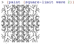
Exercise 2.52 asks us to make changes to the square limit of wave shown in figure 2.9 by working at the appropriate level of abstraction for the required change. (We'll need all the code we wrote in exercises 2.44 and 2.49 to start out with, so copy those into a new Scheme file.)

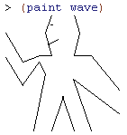
2.52a. Add some segments to the primitive wave painter of exercise 2.49 (to add a smile, for example).

This change requires that we make a change at a low level of abstraction, in adding segments to the wave painter itself. Let's add an eye and a smiling mouth on the left side of the head so it looks like the person in wave is looking in that direction.

; The wave painter (2.49d).
; Add some segments to form a smile (2.52a)
(define wave-segments
 (list
  (make-segment
   (make-vect 0.006 0.840)
   (make-vect 0.155 0.591))
  (make-segment
   (make-vect 0.006 0.635)
   (make-vect 0.155 0.392))
  (make-segment
   (make-vect 0.304 0.646)
   (make-vect 0.155 0.591))
  (make-segment
   (make-vect 0.298 0.591)
   (make-vect 0.155 0.392))
  (make-segment
   (make-vect 0.304 0.646)
   (make-vect 0.403 0.646))
  (make-segment
   (make-vect 0.298 0.591)
   (make-vect 0.354 0.492))
  (make-segment ; left face
   (make-vect 0.403 0.646)
   (make-vect 0.348 0.845))
  (make-segment
   (make-vect 0.354 0.492)
   (make-vect 0.249 0.000))
  (make-segment
   (make-vect 0.403 0.000)
   (make-vect 0.502 0.293))
  (make-segment
   (make-vect 0.502 0.293)
   (make-vect 0.602 0.000))
  (make-segment
   (make-vect 0.348 0.845)
   (make-vect 0.403 0.999))
  (make-segment
   (make-vect 0.602 0.999)
   (make-vect 0.652 0.845))
  (make-segment
   (make-vect 0.652 0.845)
   (make-vect 0.602 0.646))
  (make-segment
   (make-vect 0.602 0.646)
   (make-vect 0.751 0.646))
  (make-segment
   (make-vect 0.751 0.646)
   (make-vect 0.999 0.343))
  (make-segment
   (make-vect 0.751 0.000)
   (make-vect 0.597 0.442))
  (make-segment
   (make-vect 0.597 0.442)
   (make-vect 0.999 0.144))
  (make-segment ; eye
   (make-vect 0.395 0.916)
   (make-vect 0.410 0.916))
  (make-segment ; smile
   (make-vect 0.376 0.746)
   (make-vect 0.460 0.790))))

2.52b. Change the pattern constructed by corner-split (for example, by using only one copy of the up-split and right-split images instead of two).

For this requirement we need to work in the middle layer of abstraction. To use only one copy of the up-split and right-split images instead of two, we can simply remove the references to top-left and bottom-right that appear in the original implementation of corner-split.

(define (corner-split painter n)
 (if (= n 0)
     painter
     (let ((up (up-split painter (- n 1)))
           (right (right-split painter (- n 1)))
           (corner (corner-split painter (- n 1))))
         (beside (below painter up)
                 (below right corner)))))

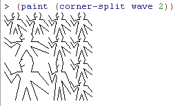
2.52c. Modify the version of square-limit that uses square-of-four so as to assemble the corners in a different pattern. (For example, you might make the big Mr. Rogers look outward from each corner of the square.)

We're not using the Mr. Rogers painter from the text, but we can still rearrange the square-limit painter so that the largest wave image is drawn in the four corners by simply rotating the corner-split painter by 180 degrees.

(define (square-limit painter n)
 (let ((quarter (rotate180 (corner-split painter n))))
   (let ((half (beside (flip-horiz quarter) quarter)))
     (below (flip-vert half) half))))

Related:

For links to all of the SICP lecture notes and exercises that I've done so far, see The SICP Challenge.

SICP 2.50 - 2.51: Transforming and Combining Painters

From SICP section 2.2.4 Example: A Picture Language

Just as we did in exercises 2.44, 2.45, and 2.49, we can use the PLT Scheme SICP Picture Language package to run the solutions to the following exercises. You can load the picture package by putting the following (require...) expression at the beginning of your Scheme file.

(require (planet "sicp.ss" ("soegaard" "sicp.plt" 2 1)))

Exercise 2.50 asks us to define the transformation flip-horiz, which flips painters horizontally, and transformations that rotate painters counterclockwise by 180 degrees and 270 degrees.

We're expected to use the transform-painter procedure defined earlier in section 2.2.4 of the text. Since we're using the PLT Scheme SICP Picture Language package, we'll be using a version of transform-painter that's defined slightly differently than the one in the text. This procedure does not take the painter to be transformed as an argument, as does the version given in the text. Instead it takes the points that specify the corners of the new frame as arguments and returns a procedure that takes the painter as its argument.

For example, instead of defining flip-vert as:

(define (flip-vert painter)
   (transform-painter painter
             (make-vect 0.0 1.0)   ; new origin
             (make-vect 1.0 1.0)   ; new end of edge1
             (make-vect 0.0 0.0))) ; new end of edge2

We would instead pass the painter as an argument to the procedure returned from transform-painter as follows:

(define (flip-vertical painter)
   ((transform-painter (make-vect 0.0 1.0)
                       (make-vect 1.0 1.0)
                       (make-vect 0.0 0.0))
    painter))

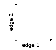
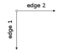
The arguments to transform-painter are points (represented as vectors) that specify the corners of the new frame. The first point specifies the new frame's origin and the other two specify the ends of its edge vectors. Remember that the origin point in a frame is normally in the lower left hand corner. The first edge vector is the bottom edge of frame and the second edge vector is the left edge of the frame.



These edges are defined by the points (0, 0) for the origin, (1, 0) for the end point of the first edge, and (0, 1) for the end point of the second edge. In order to transform a painter we just need to redraw the figure above in the desired orientation, then call transform-painter with the new positions of the origin and the end points of the edges.

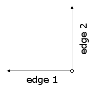
To flip a painter horizontally we just move the origin and left edge to the right.



This gives the bottom edge a new endpoint as well. The procedure (based on flip-vert) would be:

(define (flip-horizontal painter)
   ((transform-painter (make-vect 1.0 0.0)   ; origin
                       (make-vect 0.0 0.0)   ; corner1
                       (make-vect 1.0 1.0))  ; corner2
    painter))

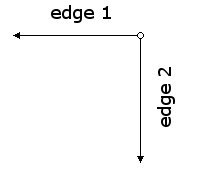
The following images show the locations of the origin and edges when we rotate an image counterclockwise by 180 and 270 degrees.





We can implement the procedures using the origin and endpoints shown in the figures above.

(define (rotate-180 painter)
   ((transform-painter (make-vect 1.0 1.0)
                       (make-vect 0.0 1.0)
                       (make-vect 1.0 0.0))
    painter))

(define (rotate-270 painter)
   ((transform-painter (make-vect 0.0 1.0)
                       (make-vect 0.0 0.0)
                       (make-vect 1.0 1.0))
    painter))

Use the einstein painter provided by the PLT Scheme SICP Picture Language package to check the output of the procedures above.




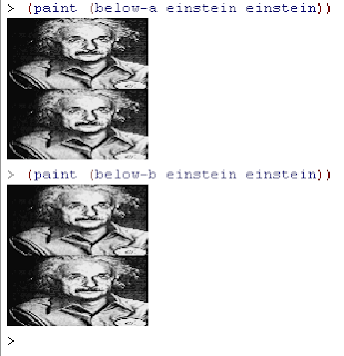
Exercise 2.51 asks us to define the below operation for painters. The below procedure takes two painters as arguments. The resulting painter draws the first painter in the bottom of the frame and the second painter in the top. We're asked to define below in two different ways -- first by writing a procedure that is analogous to the beside procedure given in the text, and again in terms of beside and suitable rotation operations like the ones we defined in exercise 2.50.

Translating the beside procedure from the text to create the first below procedure is a simple matter of applying what we learned in exercise 2.50 above.

(define (beside painter1 painter2)
   (let ((split-point (make-vect 0.5 0.0)))
   (let ((paint-left
         (transform-painter painter1
                            (make-vect 0.0 0.0)
                            split-point
                            (make-vect 0.0 1.0)))
         (paint-right
         (transform-painter painter2
                            split-point
                           (make-vect 1.0 0.0)
                           (make-vect 0.5 1.0))))
   (lambda (frame)
     (paint-left frame)
     (paint-right frame)))))

The beside procedure first defines a split-point at the bottom center of the frame that splits the frame vertically. It then transforms the two painters provided so that they each fit into one half of the frame. Finally, it returns a procedure that, when given a frame, paints the two images in the left and right halves of the frame. Here's the analogous below procedure:

; 2.51a
(define (below-a painter1 painter2)
   (let ((split-point (make-vect 0.0 0.5)))
   (let ((paint-bottom
        ((transform-painter (make-vect 0.0 0.0)
                            (make-vect 1.0 0.0)
                            split-point)
         painter1))
        (paint-top
        ((transform-painter split-point
                            (make-vect 1.0 0.5)
                            (make-vect 0.0 1.0))
         painter2)))
   (lambda (frame)
     (paint-bottom frame)
     (paint-top frame)))))

We need to redefine the split-point so that it divides the frame horizontally instead of vertically. We then transform the painters so that they fit into the bottom and top halves of the frame. Finally, we return a procedure that draws the two halves.

The second implementation of below is even simpler than the first. We just need to draw the two painters beside each other then rotate the frame by 90 degrees. When we do that the two images will be draw on their side, so we need to rotate the individual images 90 degrees in the opposite direction inside their smaller frames. This is equivalent to rotating them 270 degrees in the same direction.

; 2.51b
(define (rotate-90 painter)
 ((transform-painter (make-vect 1.0 0.0)
                     (make-vect 1.0 1.0)
                     (make-vect 0.0 0.0))
   painter))

(define (below-b painter1 painter2)
   (rotate-90 (beside (rotate-270 painter1) (rotate-270 painter2))))

Once again, we can test with einstein to verify that these two procedures both give us the desired output.




Related:

For links to all of the SICP lecture notes and exercises that I've done so far, see The SICP Challenge.

SICP 2.49: Defining Primitive Painters

From SICP section 2.2.4 Example: A Picture Language

Exercise 2.49 asks us to use segments->painter to define the following primitive painters:

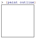
1. The painter that draws the outline of the designated frame.
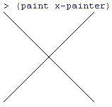
2. The painter that draws an "X'' by connecting opposite corners of the frame.
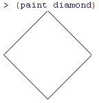
3. The painter that draws a diamond shape by connecting the midpoints of the sides of the frame.
4. The wave painter.

Just as we did in exercises 2.44 & 2.45, we can use the PLT Scheme SICP Picture Language package to run the exercises. You can load the picture package by putting the following (require...) expression at the beginning of your Scheme file.

(require (planet "sicp.ss" ("soegaard" "sicp.plt" 2 1)))

Since segments->painter takes a list of segments as its input parameter, each solution is just a matter of figuring out the coordinates of the endpoints of each required segment. Recall that the (0.0, 0.0) coordinate is the bottom left corner in the frame, not the top left corner as it is in many GUI environments. For each solution, we can define the list of segments first, then define a painter.

; 2.49 a.
; The painter that draws the outline of the designated frame.
(define outline-segments
 (list
  (make-segment
   (make-vect 0.0 0.0)
   (make-vect 0.0 0.99))
  (make-segment
   (make-vect 0.0 0.0)
   (make-vect 0.99 0.0))
  (make-segment
   (make-vect 0.99 0.0)
   (make-vect 0.99 0.99))
  (make-segment
   (make-vect 0.0 0.99)
   (make-vect 0.99 0.99))))

(define outline (segments->painter outline-segments))

Note that I used 0.99 instead of 1.0 for the edges of the frame. This is because the top and right edges won't be displayed if you use 1.0.

; 2.49 b.
; The painter that draws an ``X'' by connecting opposite corners of the frame.
(define x-segments
 (list
  (make-segment
   (make-vect 0.0 0.0)
   (make-vect 0.99 0.99))
  (make-segment
   (make-vect 0.0 0.99)
   (make-vect 0.99 0.0))))

(define x-painter (segments->painter x-segments))

; 2.49 c.
; The painter that draws a diamond shape by connecting the midpoints of the sides of the frame.
(define diamond-segments
 (list
  (make-segment
   (make-vect 0.0 0.5)
   (make-vect 0.5 0.0))
  (make-segment
   (make-vect 0.0 0.5)
   (make-vect 0.5 0.999))
  (make-segment
   (make-vect 0.5 0.999)
   (make-vect 0.999 0.5))
  (make-segment
   (make-vect 0.999 0.5)
   (make-vect 0.5 0.0))))

(define diamond (segments->painter diamond-segments))

The wave painter in the last part of the exercise is the image shown in Figure 2.10 of the text. It consists of 17 separate segments.

; 2.49 d.
; The wave painter.
(define wave-segments
 (list
  (make-segment
   (make-vect 0.006 0.840)
   (make-vect 0.155 0.591))
  (make-segment
   (make-vect 0.006 0.635)
   (make-vect 0.155 0.392))
  (make-segment
   (make-vect 0.304 0.646)
   (make-vect 0.155 0.591))
  (make-segment
   (make-vect 0.298 0.591)
   (make-vect 0.155 0.392))
  (make-segment
   (make-vect 0.304 0.646)
   (make-vect 0.403 0.646))
  (make-segment
   (make-vect 0.298 0.591)
   (make-vect 0.354 0.492))
  (make-segment
   (make-vect 0.403 0.646)
   (make-vect 0.348 0.845))
  (make-segment
   (make-vect 0.354 0.492)
   (make-vect 0.249 0.000))
  (make-segment
   (make-vect 0.403 0.000)
   (make-vect 0.502 0.293))
  (make-segment
   (make-vect 0.502 0.293)
   (make-vect 0.602 0.000))
  (make-segment
   (make-vect 0.348 0.845)
   (make-vect 0.403 0.999))
  (make-segment
   (make-vect 0.602 0.999)
   (make-vect 0.652 0.845))
  (make-segment
   (make-vect 0.652 0.845)
   (make-vect 0.602 0.646))
  (make-segment
   (make-vect 0.602 0.646)
   (make-vect 0.751 0.646))
  (make-segment
   (make-vect 0.751 0.646)
   (make-vect 0.999 0.343))
  (make-segment
   (make-vect 0.751 0.000)
   (make-vect 0.597 0.442))
  (make-segment
   (make-vect 0.597 0.442)
   (make-vect 0.999 0.144))))

(define wave (segments->painter wave-segments))

Related:

For links to all of the SICP lecture notes and exercises that I've done so far, see The SICP Challenge.

SICP 2.44 & 2.45: A Picture Language

From SICP section 2.2.4 Example: A Picture Language

The next section of SICP is an extended example that illustrates the features of the picture language introduced in SICP Lecture 3A: Henderson Escher Example. I'm going to be using the PLT Scheme SICP Picture Language package to run the examples and exercises. You can load the picture package by putting the following (require...) expression at the beginning of your Scheme file.

(require (planet "sicp.ss" ("soegaard" "sicp.plt" 2 1)))

The painter primitive in the PLT package behaves slightly differently than the one presented in the text, in that it doesn't display itself. To display a painter you must call the paint procedure, which takes a painter as its argument.

> (paint einstein)





> (paint diagonal-shading)

The einstein and diagonal-shading painter values are built in to the PLT Scheme Picture Language package. The package also includes procedures for flipping, rotating and combining painter values, similar to those discussed in the lecture.

> (paint (flip-horiz einstein))





> (paint (flip-vert einstein))





> (paint (rotate90 einstein))





> (paint (beside einstein einstein))





> (paint (below einstein einstein))

Now that we can work with painters, we can start to combine them in ways that form patterns. For example, the text shows us how we can combine an image beside a flipped representation of itself, then draw the resulting painter below itself.

(define (flipped-pairs painter)

   (let ((painter2 (beside painter (flip-vert painter))))

     (below painter2 painter2)))



> (paint (flipped-pairs einstein))

We can also define recursive operations, like right-split, which makes painters split and branch towards the right as many times as we specify.

(define (right-split painter n)

   (if (= n 0)

       painter

       (let ((smaller (right-split painter (- n 1))))

         (beside painter (below smaller smaller)))))



> (paint (right-split einstein 3))

Exercise 2.44 asks us to define the procedure up-split. It's similar to right-split, except that it switches the roles of below and beside.

(define (up-split painter n)

   (if (= n 0)

       painter

       (let ((smaller (up-split painter (- n 1))))

         (below painter (beside smaller smaller)))))



> (paint (up-split einstein 3))

Once we have both right-split and up-split defined, we can create balanced patterns by branching in both directions.

(define (corner-split painter n)

   (if (= n 0)

      painter

       (let ((up (up-split painter (- n 1)))

            (right (right-split painter (- n 1))))

         (let ((top-left (beside up up))

               (bottom-right (below right right))

               (corner (corner-split painter (- n 1))))

           (beside (below painter top-left)

                   (below bottom-right corner))))))



> (paint (corner-split einstein 1))





> (paint (corner-split einstein 2))

By combining four copies of the corner-split pattern, we can create the square-limit pattern from the Escher drawing that we saw in the lecture.

(define (square-limit painter n)

   (let ((quarter (corner-split painter n)))

     (let ((half (beside (flip-horiz quarter) quarter)))

       (below (flip-vert half) half))))



> (paint (square-limit einstein 4))

Exercise 2.45 points out that right-split and up-split can be expressed as instances of a general splitting operation. We are to define a split procedure, and then rewrite right-split and up-split in terms of split as follows:

(define right-split (split beside below))

(define up-split (split below beside))

We already noted the similarity between the two procedures right-split and up-split when we solved exercise 2.44 above. The only real difference between them is in which direction they split the painter first. Given the amount of duplication between the two, we can use either one of these procedures as a template for split.

(define (split dir1 dir2)

   (lambda (painter n)

     (if (= n 0)

         painter

         (let ((smaller ((split dir1 dir2) painter (- n 1))))

           (dir1 painter (dir2 smaller smaller))))))

The biggest change is that split uses a lambda to return the procedure that it creates. Once you're done substituting the new definitions for right-split and up-split, you can run the square-limit procedure again to verify that the output hasn't changed.


Related:

For links to all of the SICP lecture notes and exercises that I've done so far, see The SICP Challenge.

SICP Lecture 3A: Henderson Escher Example

Structure and Interpretation of Computer Programs
Henderson Escher Example
Covers Text Section 2.2.2

You can download the video lecture or stream it on MIT's OpenCourseWare site. It's also available on YouTube.

This lecture is presented by Professor Harold Abelson.

This lecture starts out with a review of the material covered in the previous lecture on compound data. The main points covered are pairs and the closure property (the things we make by forming pairs can also be combined to form pairs).

We're then shown how cons can be used to create lists of primitive elements in Scheme.

(cons 1
    (cons 2
         (cons 3
              (cons 4 nil))))

is the same as

(list 1 2 3 4)

A common pattern in programming is to write procedures that takes a list, do something to every element of that list, and return a list containing the results. We saw an example, scale-list, that takes a list and a factor and returns the result of each element in the list multiplied by the factor.

(define (scale-list items factor)
   (if (null? items)
       nil
       (cons (* (car items) factor)
             (scale-list (cdr items) factor))))

In Scheme terms, the general pattern here is to recursively do something to the cdr of the list and cons that on to actually doing something to the first element of the list.

The very fact that there's a general pattern there means I shouldn't be writing this procedure at all.

Instead of embedding a general pattern in each procedure that uses it, we should write a procedure that's the general pattern itself and write our procedure in terms of that higher-order procedure. For this example, that higher-order procedure is map. (See SICP 2.21 - 2.23: Mapping over lists for examples.)

(define (map proc items)
   (if (null? items)
       nil
       (cons (proc (car items))
             (map proc (cdr items)))))

The important idea here is that we stop thinking about control structures and start thinking about applying operations to aggregates.


Henderson Escher Example

The remainder of the lecture talks about one particular example, the Henderson Escher Example, that summarizes everything that's been covered in the course so far, list structure, abstraction, representation, and capturing commonality with higher-order procedures. It also goes into the third major theme of the course, meta-linguistic abstraction.

Meta-linguistic abstraction:

• Primitives
• Means of Combination
• Means of Abstraction

The example is a language developed by Peter Henderson for describing images that are composed of repeated elements that are shifted and scaled, like the M. C. Escher woodcut "Square Limit" pictured below.


The other theme illustrated by this example is the issue that there is no real difference between procedures and data.

The language operates on primitives called pictures. A picture is a procedure that draws a figure scaled to fit a rectangle that you specify. The following operations are supported in the language.

• rotate - Rotate a picture 90 degrees.
• flip - Flip a picture horizonally or vertically.
• beside - Draw two pictures beside one another.
• above - Draw two pictures, one above the other.

The closure property allows you to build complex pictures with just these few operations and one primitive (the picture itself). When you combine two pictures with beside or above, the result is itself a picture, which can be combined with other pictures.

We're going to see a lot of details concerning the implementation of the picture language illustrated in this example as we go through the exercises in the next section of the text, so I won't reproduce those details here. The gist is that we define one set of procedures to draw pictures inside of rectangles, another set of procedures that do the geometric manipulations of those pictures listed above (rotate, flip, beside, and above), then a higher-order set of procedures that combine those manipulated pictures in different ways to make an image like the Escher drawing above..


Software Design Methodologies

The last part of the lecture talks about the common software design methodology of decomposing a problem into discrete components, which are themselves decomposed into discrete components, and so on until you reach a design that looks like the tree structure below.


Each component in this kind of design is created to do one specific task, and the components only communicate with direct parent or child components in the hierarchy. Contrast this with the way the picture language was developed in the Henderson Escher example. First, a language for drawing primitive pictures was presented, then on top of that we build a language for geometric rotations, and finally, on top of that we built a language for schemes of combination.


This scheme gives you a full range of linguistic power at each level.

Lisp is a lousy language for doing any particular problem. What it's good for is figuring out the right language that you want and embedding that in Lisp.

For links to all of the SICP lecture notes and exercises that I've done so far, see The SICP Challenge.

SICP 2.5: Representing Pairs as a Product

From SICP section 2.1.3 What Is Meant by Data?

Exercise 2.5 asks us to show that we can represent pairs of non-negative integers using only numbers and arithmetic operations if we represent the pair a and b as the integer that is the product 2^a3^b. We're to give the corresponding definitions of the procedures cons, car, and cdr.

This exercise reminds me of the old adage that just because you can do something doesn't mean that you should. The implementations of cons, car, and cdr that follow are severely limited in that they can only join pairs of integers, not pairs of any type of data as we've seen before.

Regardless, here is what is meant by representing non-negative integers as the product 2^a3^b. Note that because 2 and 3 are both prime, and due to the fundamental theorem of arithmetic, any integer values that we insert for a and b will result in a unique value for the product 2^a3^b. Because the product is unique, we're able to get back the original values of a and b by just storing the product and remembering the rule we used to generate it.

The definition of cons is straightforward from the requirements using the built-in Scheme expt procedure.

(define (cons a b)
  (* (expt 2 a)
     (expt 3 b)))

But once we've combined two integers in this way, how do we separate them again? For example, if we evaluate (cons 5 6) we get a result of 23328. The corresponding implementation of car needs to take the value 23328 and tell us what that the original value of a was 5. We can do that by counting the number of times 23328 is evenly divisible by 2. Since 2 and 3 have no factors in common, once you divide all the 2s out of 23328 you'll be left with a power of 3. Since we're going to be doing the same thing for cdr, we'll define a general procedure that can be reused.

There's no easy way to find out how many times one number evenly divides another other than simply trying to divide by the number in a loop and testing for a remainder. If there was a quick formula that we could apply to get the answer in one step then prime factorization would be much easier than it is. We'll have to use an iterator to do this in as few steps as possible.

; count the number of times n is evenly divisible by d
(define (num-divs n d)
  (define (iter x result)
    (if (= 0 (remainder x d))
        (iter (/ x d) (+ 1 result))
        result))
  (iter n 0))

I tested this with the example values above to make sure it gives the correct results.

> (num-divs 23328 2)
5
> (num-divs 23328 3)
6

Now we can define both car and cdr in terms of num-divs.

(define (car x)
  (num-divs x 2))

(define (cdr x)
  (num-divs x 3))

Finally, we can use the axiom of pairs (from Lecture 2B) to show that our new definitions for cons, car, and cdr work together as they should.

> (car (cons 4 7))
4
> (cdr (cons 4 7))
7

Related:

For links to all of the SICP lecture notes and exercises that I've done so far, see The SICP Challenge.

SICP Lecture 2B: Compound Data

Structure and Interpretation of Computer Programs
Compound Data
Covers Text Section 2.1: Introduction to Data Abstraction

You can download the video lecture or stream it on MIT's OpenCourseWare site. It's also available on YouTube.

This lecture is presented by Professor Harold Abelson

Chapter 1 of SICP was all about procedures using primitive data, and how to build higher and higher abstractions using procedures. The next chapter will be all about combining primitive data into compound data abstractions.

The fundamental means of combining primitive data in Scheme is to glue two things together into a pair. We use the cons function to combine two things together to make a pair. Once you've combined them you need something to get the two separate parts back. To do that you use the car and cdr functions.

(cons x y) - constructs a pair whose first part is x and second part is y.

(car p) - selects the first part of the pair p.

(cdr p) - selects the second part of the pair p.

The convention for drawing diagrams of pairs is called box-and-pointer notation.




The formal way of describing the behavior of cons, car, and cdr, and how they interact with one another is called the axiom for pairs:

For any x and y:
(car (cons x y)) is x
(cdr (cons x y)) is y

Representing rational numbers

The text defines a system for representing rational numbers using pairs.

(define (make-rat n d) (cons n d))

(define (numer x) (car x))
(define (denom x) (cdr x))

These functions are called a constructor (make-rat) and selectors (numer and denom). Once we have the simple data abstraction in place, we can use the abstraction to define other procedures that work with rational numbers using the rules of rational number arithmetic.

(define (add-rat x y)
   (make-rat (+ (* (numer x) (denom y))
                (* (numer y) (denom x)))
             (* (denom x) (denom y))))

(define (sub-rat x y)
   (make-rat (- (* (numer x) (denom y))
                (* (numer y) (denom x)))
             (* (denom x) (denom y))))

(define (mul-rat x y)
   (make-rat (* (numer x) (numer y))
             (* (denom x) (denom y))))

(define (div-rat x y)
   (make-rat (* (numer x) (denom y))
             (* (denom x) (numer y))))

(define (print-rat x)
   (newline)
   (display (numer x))
   (display "/")
   (display (denom x)))

Data abstraction separates the use of a data object from its representation. You could define add-rat and the other procedures without using data abstraction by directly using cons, car, and cdr. The point of isolating the use from the representation is that you have to capture the idea of a conceptual entity.


Compound Data

Like procedure definition, the real power of compound data is that we can use it to create building blocks that can themselves be used to create more complex data structures. Using the same method we used for creating rational numbers, we could also create a set of functions for representing points in a plane. From those points we can build line segments, from line segments we can build two-dimensional shapes. We could keep going and build as many abstractions on top of each other as we need to represent any system we want.

Closure - the means of combination in the system are such that when you put things together with them you can then put those things together using the same means. The system is closed. (This use of the word "closure" is in the same sense as it's used in abstract algebra. The Lisp community also uses the same word for an unrelated concept.)

Once you can combine two things, the closure property allows you to combine as many things as you want.



We'll see later in the text that this is how lists are formed in Scheme.


What are pairs really?

The last section of the lecture shows that pairs can be build out of nothing at all. If Scheme didn't have primitive functions cons, car, and cdr we could define them ourselves.

(define (cons a b)
  (lambda (pick)
     (cond ((= pick 1) a)
           ((= pick 2) b))))

(define (car x) (x 1))
(define (cdr x) (x 2))

In this implementation cons returns a procedure, not a pair. The definitions for car and cdr take the procedure supplied by cons and apply it to 1 and 2 respectively. If this system satisfies the axiom for pairs that we saw earlier, then it's a perfectly reasonable implementation. In the lecture, mechanical substitution is used to prove that this system does satisfy the axiom for pairs.


Related:

For links to all of the SICP lecture notes and exercises that I've done so far, see The SICP Challenge.

SICP Lecture 2A: Higher-order Procedures

Structure and Interpretation of Computer Programs
Higher-order Procedures
Covers Text Section 1.3

You can download the video lecture or stream it on MIT's OpenCourseWare site. It's also available on YouTube.

This lecture is presented by MIT's Professor Gerald Jay Sussman.

Introduction

So far in the SICP lectures and exercises, we've seen that we can use procedures to describe compound operations on numbers. This is a first-order abstraction. Instead of performing primitive operations on the values to solve a distinct instance of a problem, we can write a procedure that performs the correct operations, then tell it what numbers to operate on when we need it. For example, instead of writing (* 5 5) when we want to find the value of 5 squared, we can define the square procedure:

(define (square x) (* x x))

then just invoke it on any number we need to square.

In this section we'll start to think about higher-order procedures. Instead of simply manipulating data (or more precisely, what we are used to thinking of as data), as in the procedures we've written so far, higher-order procedures manipulate other procedures by accepting them as arguments or returning them as values.

Procedures as Arguments

The video lecture explains this concept by looking at three very similar procedures, then showing how one idea can be refactored out of them to create a procedure that can be reused. The three procedures are the sum of the integers from a to b, the sum of the squares from a to b (the text book uses the sum of cubes), and Leibniz's formula for finding π/8.

(define (sum-int a b)
 (if (> a b)
     0
     (+ a (sum-int (+ a 1) b))))

(define (sum-sq a b)
  (if (> a b)
      0
      (+ (square a) (sum-sq (+ a 1) b))))

(define (pi-sum a b)
  (if (> a b)
      0
      (+ (/ 1.0 (* a (+ a 2)))
         (pi-sum (+ a 4) b))))

As you can see, these procedures are all nearly identical. The only things that are different are the function being applied to each term in the sequence, how you get to the next term of the sequence, and the names of the procedures themselves. We can use the similarities of these procedures to create a general pattern that describes all three.

(define (<name> a b)
  (if (> a b)
      0
      (+ <term> (<name> (<next> a) b))))

The general pattern is that the procedure:

• is given a name
• takes two arguments (a lower bound and an upper bound)
• performs a test to see if the upper bound is exceeded
• applies some procedure to the current term and adds the result to the recursive call to get the next term
• computes of the next term

The important thing to note here is that some of the things that change are procedures, not just numbers.

There's nothing very special about numbers. Numbers are just one kind of data.

Since procedures are also a type of data in Scheme, we can use them as arguments to other procedures as well. Now that we have a general pattern, we use it to define a sigma procedure.

(define (sum term a next b)
  (if (> a b)
      0
      (+ (term a)
         (sum term (next a) next b))))

The arguments term and next are procedures that are passed in to the sum procedure, and will be used to compute the value of the current term and how to get to the next one.

We can use the procedure above to rewrite sum-int as follows:

(define (sum-int a b)
  (define (identity x) x)
  (sum identity a inc b))

First, the identity procedure simply takes an argument and returns that argument. We need this because the sum-int procedure doesn't apply any function to each term of the sequence, it just sums up the raw terms. Our sum procedure is expecting a procedure as its second argument, so we have to give it one. Next we simply call the sum procedure, passing in the identity and increment procedures for term and next.

The sum-sq and pi-sum procedures can be rewritten as well (which is kind of the point).

(define (sum-sq a b)
  (define (identity x) x)
  (sum square a inc b))

(define (pi-sum a b)
  (sum (lambda (i) (/ 1.0 (* x (+ x 2))))
       a
       (lambda (i) (+ x 4))
       b))

Note that in the pi-sum example, we use lambda notation to define the procedures for term and next as we are passing them in to sum. We can redefine pi-sum without lambda notation by explicitly defining named procedures.

(define (pi-sum a b)
  (define (pi-term x)
     (/ 1.0 (* x (+ x 2))))
  (define (pi-next x)
     (+ x 4))
  (sum pi-term a pi-next b))

This makes no difference in how the code is evaluated. In the first example we passed a procedure by its definition, in the second we passed it by its name. In future articles on lectures and exercises, I'll be using more and more lambda notation since we should be becoming more familiar with it.

Separating the abstract idea of sum into its own procedure allows us to reuse it in several situations where that idea is needed. Another important point is that we could reimplement sum itself, in perhaps a more efficient way, and we would benefit from it everywhere it is used without having to rewrite all the procedures that use it. Here's an iterative implementation of sum.

(define (sum term a next)
  (define (iter j ans)
      (if (> j b)
          ans
          (iter (next j)
                (+ (term j) ans))))
  (iter a 0))

Decomposing procedures in this way allows us to change one abstraction without needing to change the every procedure where it is used. If we wanted to use the iterative approach to summation in the original three procedures at the top, we'd have to rewrite all three of them individually. Putting the summation code in its own procedure allows you to change it in one place, but use it everywhere the procedure is called.


Abstraction

In section 1.1.8 we looked at Heron of Alexandria's method for computing a square root.

(define (sqrt x)
  (define tolerance 0.00001)
  (define (good-enough? y)
     (< (abs (- (* y y) x)) tolerance ))
  (define (improve y)
     (average (/ x y) y))
  (define (try y)
     (if (good-enough? y)
         y
        (try (improve y))))
  (try 1))

The algorithm for computing the square root of x is not intuitively obvious from looking at the code in this procedure. In this section we'll show how abstraction can be used to clarify how this procedure works.

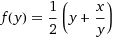
The procedure iteratively improves a guess until it is within a pre-defined tolerance of the correct answer. The function for improving the guess for the square root of x is to average the guess with x divided by x. In mathematical terms


If you substitute in √x for y, you'll notice that we're looking for a fixed point of this function. (A fixed point of a function is a point that is mapped to itself by the function. If you put a fixed point into a function, you get the same value out.)

f(y) = (y + x/y) / 2
f(√x) = (√x + x/√x) / 2
f(√x) = (√x + √x) / 2
f(√x) = 2 * √x / 2
f(√x) = √x

We can use this to rewrite the sqrt procedure in terms of computing a fixed point. (Even though we don't have a procedure to compute a fixed point yet. That will be coming up next.)

(define (sqrt x)
  (fixed-point
      (lambda (y) (average (/ x y) y))
      1))

This procedure shows how to compute the square root of x in terms of computing a fixed point, but from this we only know that what we pass to the fixed-point procedure is another procedure and an initial guess. At this point, fixed-point is only "wishful thinking." Here's one way to compute fixed points of a function:

(define (fixed-point f start)
  (define tolerance 0.00001)
  (define (close-enuf? u v)
     (< (abs (- u v)) tolerance))
  (define (iter old new)
     (if (close-enuf? old new)
         new
         (iter new (f new))))
  (iter start (f start)))

This procedure computes:

the fixed point of the function computed by the procedure whose name will be "f" in this procedure.

This is a key quote from the lecture because it illustrates how procedures can treated like any other data in Scheme. Here, the variable f can take on the value of any procedure you want to pass in.

The fixed point of the function passed in to fixed-point is computed by iteratively applying the function to its own result, starting at the initial guess, until the change in the result is smaller than some tolerance. Note how the function that is passed in as the parameter f is evaluated in the iteration loop.

If you define an average procedure you can run the new sqrt procedure in a Scheme interpreter to test it out.

(define (average x y)
  (/ (+ x y) 2))

Procedures as Returned Values

There's another abstraction that we can pull out of the previous fixed-point procedure. Before we get to that, a simpler procedure for computing functions whose fixed point is the square root is:

g(y) = x/y

This has the same property as the function we looked at before, if you insert √x in for y, you get √x back. The reason that we didn't use this simpler function before is that for some inputs it will oscillate. If x is 2, and your initial guess is 1, then the old and new values will oscillate between 2 and 1, never getting any closer together. The original function that uses the average procedure is just damping out this oscillation. We can pull this damping concept out by first defining sqrt as a function of a fixed-point procedure that is itself a function of average damping.

(define (sqrt x)
  (fixed-point
      (average-damp (lambda (y) (/ x y)))
      1))

Here, average-damp takes a procedure as its argument and returns a procedure as its value. When given a procedure that takes an argument, average-damp returns another procedure that computes the average of the values before and after applying the original procedure to its argument.

(define average-damp
  (lambda (f)
      (lambda (x) (average (f x) x))))

This is special because it's the first time we've seen a procedure that produces a procedure as its result.


Newton's method

A general method for finding roots (zeroes) of functions is called Newton's method. To find a y such that

f(y) = 0

the general procedure is to start with a guess y₀, then iterate the following expression using the function:

y_n+1 = y_n - f(y_n) / df/dy | y = y_n

This is a difference equation. Each term is the difference between the previous term and the function applied to the previous term divided by the derivative with respect to y of f evaluated at the previous term. (The Scheme representation of this should be a lot more clear, but for now we just need to remember that the derivative of f with respect to y is a function.) We'll start the same way we did before, by applying the method before we define it.

We can define sqrt in terms of Newton's method as follows:

(define (sqrt x)
  (newton (lambda (y) (- x (square y)))
          1))

The square root of x is computed by applying Newton's method to the function of y that computes the difference between x and the square of y. If we had a value of y for which the difference between x and y² returned 0, then y would be the square root of x.

Now we have to define a procedure for Newton's method. Note that we're still using a method of iteratively improving a guess, just as we did in the earlier sqrt procedures. Look again at the expression for Newton's method:

y_n+1 = y_n - f(y_n) / df/dy | y = y_n

We'd like to find some value for y_n such that when we plug it in on the right hand side of this expression, we get the same value back out on the left hand side (within some small tolerance). So once again, we are looking for a fixed point.

(define (newton f guess)
  (define df (deriv f))
  (fixed-point
      (lambda (x) (- x (/ (f x) (df x))))
      guess))

This procedure takes a function and an initial guess, and computes the fixed point of the function that computes the difference of x and the quotient of the function of x and the derivative of the function of x.

Wishful thinking is essential to good engineering, and certainly essential to good computer science.

Along the way we have to write a procedure that computes the derivative (a function) of the function passed to it.

(define deriv
  (lambda (f)
      (lambda (x)
          (/ (- (f (+ x dx))
             (f x))
          dx))))

(define dx 0.0000001)

You may remember from Calculus or a past life that the derivative of a function is the function of x that computes

f(x + Δx) - f(x) / Δx

for some small value of Δx. You might also remember (and perhaps a bit more readily) that the derivative of x² is 2x. So if we apply our deriv procedure to square, we should expect to get back a procedure that computes 2x. Unfortunately when I tried it in a Scheme interpreter I got back:

> (deriv square)
#<procedure>

That's not very revealing, so we're not done experimenting yet. How can we figure out what that returned procedure does? Let's just apply it to some values.

> ((deriv square) 2)
4.000000091153311
> ((deriv square) 5)
10.000000116860974
> ((deriv square) 10)
19.999999949504854
> ((deriv square) 25)
50.00000101063051
> ((deriv square) 100)
199.99999494757503

That looks like a fair approximation to the expected procedure.


Abstractions and first-class procedures

The lecture wraps up with the following list by computer scientist Christopher Strachey, one of the inventors of denotational semantics.

The rights and privileges of first-class citizens:

• To be named by variables.
• To be passed as arguments to procedures.
• To be returned as values of procedures.
• To be incorporated into data structures.

We've seen that both values and procedures in Scheme meet the first three requirements. In later sections we'll see that they both meet the fourth requirement as well.

Having procedures as first class data allows us to make powerful abstractions that encode general methods like Newton's method in a very clear way.

For links to all of the SICP lecture notes and exercises that I've done so far, see The SICP Challenge.