The "N Days of Christmas" Solution

A few days ago in The "N Days of Christmas" Puzzle I asked if you could figure out how many gifts you receive in total for all twelve days (not just on the twelfth day) of the song "The Twelve Days of Christmas," and to find an elegant way to calculate the number of gifts you'd receive if the number of days is extended beyond twelve.

First we need to figure out how many gifts we receive on a given day. It is a cumulative song, so you receive one partridge in a pear tree on the first day, then on the second day you receive two turtle doves and another partridge in a pear tree, and so on for twelve days. So the sequence for each day is:

1
1 + 2 = 3
1 + 2 + 3 = 6
1 + 2 + 3 + 4 = 10
1 + 2 + 3 + 4 + 5 = 15
...

That's probably enough terms that you'll start to recognize a pattern is forming. Each number in the sequence is just the sum of the first n integers, which you may recognize as the triangle numbers. For a small number of days like 12 we can just continue adding terms to the sequence and have the answer in about a minute. We could look up the formula for the nth triangle number, but with a little bit of intuition we can come up with one ourselves. (When you write your own blog, you get to pretend you're a little bit smarter and less lazy than you really are.) Sometimes it helps to draw a picture like the following:



Notice that the circles form the same sequence that we're after. Also note that since the circles are arranged in a triangle we can calculate the total number of circles by multiplying the height of the enclosing rectangle (n) by the width (n + 1) and dividing by 2. This gives us the formula for the nth triangle number.

$T_n = \frac{n(n + 1)}{2}$

That only gives us the number of gifts on the last day though. We wanted to know the number of gifts on all days combined, and we wanted to know it for any number of days. So what we really want isn't the nth triangle number (the sum of the first n integers), but the sum of the first n triangle numbers. That's a formula that we can derive from what we already know.

$\sum_{k=1}^{n}\frac{k(k + 1)}{2}$

$\frac{1}{2}\sum_{k=1}^{n}k(k + 1)$

$\frac{1}{2}\sum_{k=1}^{n}(k^2 + k)$

$\frac{1}{2}\sum_{k=1}^{n}k^2 + \frac{1}{2}\sum_{k=1}^{n}k$

At this point we should take a moment to say out loud what the two terms in this equation mean in plain English. On the left we have one-half of the sum of the first n squares, and on the right we have one-half of the sum of the first n integers. We already found a formula for the sum of the first n integers, and it seems like there ought to be a similar formula for the sum of the first n squares. There is, and to save us some time I’ll just substitute it here¹.

$\frac{1}{2}\frac{n (n + 1) (2n + 1)}{6} + \frac{1}{2}\frac{n (n + 1)}{2}$

$\frac{(n^2 + n)(2n + 1)}{12} + \frac{n(n + 1)}{4}$

$\frac{(2n^3 + 3n^2 + n)}{12} + \frac{(n^2 + n)}{4}$

$\frac{(2n^3 + 3n^2 + n)}{12} + \frac{(3n^2 + 3n)}{12}$

$\frac{(2n^3 + 6n^2 + 4n)}{12}$

$\frac{(n^3 + 3n^2 + 2n)}{6}$

$\frac{n(n^2 + 3n + 2)}{6}$

$\frac{n(n + 1)(n + 2)}{6}$

That gives us our formula for the sum of the first n triangle numbers, which is also known as a tetrahedral number. This is the number you get when you turn the first n triangles on their side and stack them in a pyramid.

So if we plug 12 into the formula above, we find out that in total there are

$\frac{12 \times 13 \times 14}{6} = 364$

total gifts given in the Twelve Days of Christmas.

Happy Holidays!

---

¹ The sequence given by the sum of the first N squares is called the square pyramidal numbers.

The "N Days of Christmas" Puzzle

I received an interesting puzzle in an email from my friend Tim recently. See if you can figure it out.

My dad and I were bored at a Christmas concert lately, so we started
talking about how many items you receive in the 12 days of Christmas.

You get 1 item on day 1, 3 items on day 2, 6 on day 3, etc. We
figured that out pretty easily, but then we were trying to come up
with a closed form solution for any number of days.

When I got home and had some paper to work with I managed to do it,
but I felt like my approach wasn't very nice.

So, can you find a solution, and more importantly do you know an
elegant way to do it?

If you're not familiar with the song, you can find the basic structure of the lyrics on Wikipedia, or just Google "the 12 days of Christmas" and you'll find it.

Just to be clear, it is a cumulative song, so you receive one partridge in a pear tree on the first day, then on the second day you receive two turtle doves and another partridge in a pear tree, for a total of four items on the first two days, and so on for twelve days. The puzzle is to find out how many gifts you receive in total for all twelve days (not just on the twelfth day), and to find an elegant way to calculate the number of gifts you'd receive if the number of days is extended beyond twelve.

You can see the solution here.

SICP 2.49: Defining Primitive Painters

From SICP section 2.2.4 Example: A Picture Language

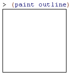
Exercise 2.49 asks us to use segments->painter to define the following primitive painters:

1. The painter that draws the outline of the designated frame.
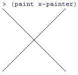
2. The painter that draws an "X'' by connecting opposite corners of the frame.
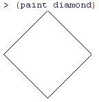
3. The painter that draws a diamond shape by connecting the midpoints of the sides of the frame.
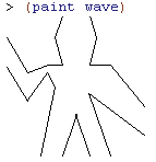
4. The wave painter.

Just as we did in exercises 2.44 & 2.45, we can use the PLT Scheme SICP Picture Language package to run the exercises. You can load the picture package by putting the following (require...) expression at the beginning of your Scheme file.

(require (planet "sicp.ss" ("soegaard" "sicp.plt" 2 1)))

Since segments->painter takes a list of segments as its input parameter, each solution is just a matter of figuring out the coordinates of the endpoints of each required segment. Recall that the (0.0, 0.0) coordinate is the bottom left corner in the frame, not the top left corner as it is in many GUI environments. For each solution, we can define the list of segments first, then define a painter.

; 2.49 a.
; The painter that draws the outline of the designated frame.
(define outline-segments
 (list
  (make-segment
   (make-vect 0.0 0.0)
   (make-vect 0.0 0.99))
  (make-segment
   (make-vect 0.0 0.0)
   (make-vect 0.99 0.0))
  (make-segment
   (make-vect 0.99 0.0)
   (make-vect 0.99 0.99))
  (make-segment
   (make-vect 0.0 0.99)
   (make-vect 0.99 0.99))))

(define outline (segments->painter outline-segments))

Note that I used 0.99 instead of 1.0 for the edges of the frame. This is because the top and right edges won't be displayed if you use 1.0.

; 2.49 b.
; The painter that draws an ``X'' by connecting opposite corners of the frame.
(define x-segments
 (list
  (make-segment
   (make-vect 0.0 0.0)
   (make-vect 0.99 0.99))
  (make-segment
   (make-vect 0.0 0.99)
   (make-vect 0.99 0.0))))

(define x-painter (segments->painter x-segments))

; 2.49 c.
; The painter that draws a diamond shape by connecting the midpoints of the sides of the frame.
(define diamond-segments
 (list
  (make-segment
   (make-vect 0.0 0.5)
   (make-vect 0.5 0.0))
  (make-segment
   (make-vect 0.0 0.5)
   (make-vect 0.5 0.999))
  (make-segment
   (make-vect 0.5 0.999)
   (make-vect 0.999 0.5))
  (make-segment
   (make-vect 0.999 0.5)
   (make-vect 0.5 0.0))))

(define diamond (segments->painter diamond-segments))

The wave painter in the last part of the exercise is the image shown in Figure 2.10 of the text. It consists of 17 separate segments.

; 2.49 d.
; The wave painter.
(define wave-segments
 (list
  (make-segment
   (make-vect 0.006 0.840)
   (make-vect 0.155 0.591))
  (make-segment
   (make-vect 0.006 0.635)
   (make-vect 0.155 0.392))
  (make-segment
   (make-vect 0.304 0.646)
   (make-vect 0.155 0.591))
  (make-segment
   (make-vect 0.298 0.591)
   (make-vect 0.155 0.392))
  (make-segment
   (make-vect 0.304 0.646)
   (make-vect 0.403 0.646))
  (make-segment
   (make-vect 0.298 0.591)
   (make-vect 0.354 0.492))
  (make-segment
   (make-vect 0.403 0.646)
   (make-vect 0.348 0.845))
  (make-segment
   (make-vect 0.354 0.492)
   (make-vect 0.249 0.000))
  (make-segment
   (make-vect 0.403 0.000)
   (make-vect 0.502 0.293))
  (make-segment
   (make-vect 0.502 0.293)
   (make-vect 0.602 0.000))
  (make-segment
   (make-vect 0.348 0.845)
   (make-vect 0.403 0.999))
  (make-segment
   (make-vect 0.602 0.999)
   (make-vect 0.652 0.845))
  (make-segment
   (make-vect 0.652 0.845)
   (make-vect 0.602 0.646))
  (make-segment
   (make-vect 0.602 0.646)
   (make-vect 0.751 0.646))
  (make-segment
   (make-vect 0.751 0.646)
   (make-vect 0.999 0.343))
  (make-segment
   (make-vect 0.751 0.000)
   (make-vect 0.597 0.442))
  (make-segment
   (make-vect 0.597 0.442)
   (make-vect 0.999 0.144))))

(define wave (segments->painter wave-segments))

Related:

For links to all of the SICP lecture notes and exercises that I've done so far, see The SICP Challenge.

SICP 2.46 - 2.48: Frames & Painters

From SICP section 2.2.4 Example: A Picture Language

A frame can be described by three vectors -- an origin vector and two edge vectors. The origin vector specifies the offset of the frame's origin from some absolute origin in the plane, and the edge vectors specify the offsets of the frame's corners from its origin. If the edges are perpendicular, the frame will be rectangular. Otherwise the frame will be a more general parallelogram. A two-dimensional vector v running from the origin to a point can be represented as a pair consisting of an x-coordinate and a y-coordinate.

Exercise 2.46 asks us to implement a data abstraction for vectors by giving a constructor make-vect and corresponding selectors xcor-vect and ycor-vect. In terms of these selectors and constructor, we'll also implement procedures add-vect, sub-vect, and scale-vect that perform the operations for vector addition, vector subtraction, and multiplying a vector by a scalar:

(x1, y1) + (x2, y2) = (x1 + x2, y1 + y2)
(x1, y1) - (x2, y2) = (x1 - x2, y1 - y2)
s * (x, y) = (sx, sy)

The solution for the constructor and selectors uses cons, car, and cdr in the same pattern we've seen at least a dozen times by now.

(define (make-vect x y)
   (cons x y))

(define (xcor-vect v)
   (car v))

(define (ycor-vect v)
   (cdr v))

Once we have those procedures in place, we can use them to build the vector operations specified.

(define (add-vect u v)
   (make-vect
     (+ (xcor-vect u) (xcor-vect v))
     (+ (ycor-vect u) (ycor-vect v))))

(define (sub-vect u v)
   (make-vect
     (- (xcor-vect u) (xcor-vect v))
     (- (ycor-vect u) (ycor-vect v))))

(define (scale-vect s v)
   (make-vect
     (* s (xcor-vect v))
     (* s (ycor-vect v))))

We can test these procedures out with a few known values before moving on to the next step.

> (define u (make-vect 2 4))
> u
(2 . 4)
> (define v (make-vect 3 1))
> v
(3 . 1)
> (define w (add-vect u v))
> w
(5 . 5)
> (define x (sub-vect w u))
> x
(3 . 1)
> (define y (scale-vect 3 w))
> y
(15 . 15)

Exercise 2.47 gives us the following constructors for frames, one using list and the other using cons:

(define (make-frame origin edge1 edge2)
   (list origin edge1 edge2))

(define (make-frame origin edge1 edge2)
   (cons origin (cons edge1 edge2)))

We're asked to supply the appropriate selectors to produce an implementation for frames for each of the two constructors. Like any selector implementation, the task here is simply to extract each piece from the assembled object. We'll follow the naming convention from the previous exercise and call our selectors origin-frame, edge1-frame, and edge2-frame. Let's start with the version that uses list.

; 2.47a
(define (make-frame origin edge1 edge2)
   (list origin edge1 edge2))

(define (origin-frame frame)
   (car frame))

(define (edge1-frame frame)
   (car (cdr frame)))

(define (edge2-frame frame)
   (car (cdr (cdr frame))))

The selectors simply use the right combinations of car and cdr to extract the appropriate elements from the list. We can test it with some of the same values used in the previous exercise, but we'll need to add an origin vector.

> (define f (make-frame (make-vect 0 0) (make-vect 2 4) (make-vect 3 1)))
> f
((0 . 0) (2 . 4) (3 . 1))
> (origin-frame f)
(0 . 0)
> (edge1-frame f)
(2 . 4)
> (edge2-frame f)
(3 . 1)

Because the internal representation of a frame is different in the second implementation of make-frame, one of the selectors will have to change for the second part of the exercise. The original origin-frame and edge1-frame implementations will still work, but the edge2-frame procedure causes an error if you try to use it.

; 2.47b
(define (make-frame origin edge1 edge2)
   (cons origin (cons edge1 edge2)))

(define (edge2-frame frame)
   (cdr (cdr frame)))

Run exactly the same test from above to verify that you get the same results (except for the internal structure of the frame in the second step).

> (define f (make-frame (make-vect 0 0) (make-vect 2 4) (make-vect 3 1)))
> f
((0 . 0) (2 . 4) 3 . 1)
> (origin-frame f)
(0 . 0)
> (edge1-frame f)
(2 . 4)
> (edge2-frame f)
(3 . 1)

Exercise 2.48 asks us to define a representation for segments using our vector representation from exercise 2.46 above. We'll need to define the constructor make-segment and the selectors start-segment and end-segment.

(define (make-segment v1 v2)
   (cons v1 v2))

(define (start-segment segment)
   (car segment))

(define (end-segment segment)
   (cdr segment))

Again, these use the same pattern we've seen before. In the next exercise, we'll take a closer look at the procedures above by drawing pictures with line segments using The SICP Picture Language package.


Related:

For links to all of the SICP lecture notes and exercises that I've done so far, see The SICP Challenge.

SICP 2.44 & 2.45: A Picture Language

From SICP section 2.2.4 Example: A Picture Language

The next section of SICP is an extended example that illustrates the features of the picture language introduced in SICP Lecture 3A: Henderson Escher Example. I'm going to be using the PLT Scheme SICP Picture Language package to run the examples and exercises. You can load the picture package by putting the following (require...) expression at the beginning of your Scheme file.

(require (planet "sicp.ss" ("soegaard" "sicp.plt" 2 1)))

The painter primitive in the PLT package behaves slightly differently than the one presented in the text, in that it doesn't display itself. To display a painter you must call the paint procedure, which takes a painter as its argument.

> (paint einstein)





> (paint diagonal-shading)

The einstein and diagonal-shading painter values are built in to the PLT Scheme Picture Language package. The package also includes procedures for flipping, rotating and combining painter values, similar to those discussed in the lecture.

> (paint (flip-horiz einstein))





> (paint (flip-vert einstein))





> (paint (rotate90 einstein))





> (paint (beside einstein einstein))





> (paint (below einstein einstein))

Now that we can work with painters, we can start to combine them in ways that form patterns. For example, the text shows us how we can combine an image beside a flipped representation of itself, then draw the resulting painter below itself.

(define (flipped-pairs painter)

   (let ((painter2 (beside painter (flip-vert painter))))

     (below painter2 painter2)))



> (paint (flipped-pairs einstein))

We can also define recursive operations, like right-split, which makes painters split and branch towards the right as many times as we specify.

(define (right-split painter n)

   (if (= n 0)

       painter

       (let ((smaller (right-split painter (- n 1))))

         (beside painter (below smaller smaller)))))



> (paint (right-split einstein 3))

Exercise 2.44 asks us to define the procedure up-split. It's similar to right-split, except that it switches the roles of below and beside.

(define (up-split painter n)

   (if (= n 0)

       painter

       (let ((smaller (up-split painter (- n 1))))

         (below painter (beside smaller smaller)))))



> (paint (up-split einstein 3))

Once we have both right-split and up-split defined, we can create balanced patterns by branching in both directions.

(define (corner-split painter n)

   (if (= n 0)

      painter

       (let ((up (up-split painter (- n 1)))

            (right (right-split painter (- n 1))))

         (let ((top-left (beside up up))

               (bottom-right (below right right))

               (corner (corner-split painter (- n 1))))

           (beside (below painter top-left)

                   (below bottom-right corner))))))



> (paint (corner-split einstein 1))





> (paint (corner-split einstein 2))

By combining four copies of the corner-split pattern, we can create the square-limit pattern from the Escher drawing that we saw in the lecture.

(define (square-limit painter n)

   (let ((quarter (corner-split painter n)))

     (let ((half (beside (flip-horiz quarter) quarter)))

       (below (flip-vert half) half))))



> (paint (square-limit einstein 4))

Exercise 2.45 points out that right-split and up-split can be expressed as instances of a general splitting operation. We are to define a split procedure, and then rewrite right-split and up-split in terms of split as follows:

(define right-split (split beside below))

(define up-split (split below beside))

We already noted the similarity between the two procedures right-split and up-split when we solved exercise 2.44 above. The only real difference between them is in which direction they split the painter first. Given the amount of duplication between the two, we can use either one of these procedures as a template for split.

(define (split dir1 dir2)

   (lambda (painter n)

     (if (= n 0)

         painter

         (let ((smaller ((split dir1 dir2) painter (- n 1))))

           (dir1 painter (dir2 smaller smaller))))))

The biggest change is that split uses a lambda to return the procedure that it creates. Once you're done substituting the new definitions for right-split and up-split, you can run the square-limit procedure again to verify that the output hasn't changed.


Related:

For links to all of the SICP lecture notes and exercises that I've done so far, see The SICP Challenge.

SICP Lecture 3A: Henderson Escher Example

Structure and Interpretation of Computer Programs
Henderson Escher Example
Covers Text Section 2.2.2

You can download the video lecture or stream it on MIT's OpenCourseWare site. It's also available on YouTube.

This lecture is presented by Professor Harold Abelson.

This lecture starts out with a review of the material covered in the previous lecture on compound data. The main points covered are pairs and the closure property (the things we make by forming pairs can also be combined to form pairs).

We're then shown how cons can be used to create lists of primitive elements in Scheme.

(cons 1
    (cons 2
         (cons 3
              (cons 4 nil))))

is the same as

(list 1 2 3 4)

A common pattern in programming is to write procedures that takes a list, do something to every element of that list, and return a list containing the results. We saw an example, scale-list, that takes a list and a factor and returns the result of each element in the list multiplied by the factor.

(define (scale-list items factor)
   (if (null? items)
       nil
       (cons (* (car items) factor)
             (scale-list (cdr items) factor))))

In Scheme terms, the general pattern here is to recursively do something to the cdr of the list and cons that on to actually doing something to the first element of the list.

The very fact that there's a general pattern there means I shouldn't be writing this procedure at all.

Instead of embedding a general pattern in each procedure that uses it, we should write a procedure that's the general pattern itself and write our procedure in terms of that higher-order procedure. For this example, that higher-order procedure is map. (See SICP 2.21 - 2.23: Mapping over lists for examples.)

(define (map proc items)
   (if (null? items)
       nil
       (cons (proc (car items))
             (map proc (cdr items)))))

The important idea here is that we stop thinking about control structures and start thinking about applying operations to aggregates.


Henderson Escher Example

The remainder of the lecture talks about one particular example, the Henderson Escher Example, that summarizes everything that's been covered in the course so far, list structure, abstraction, representation, and capturing commonality with higher-order procedures. It also goes into the third major theme of the course, meta-linguistic abstraction.

Meta-linguistic abstraction:

• Primitives
• Means of Combination
• Means of Abstraction

The example is a language developed by Peter Henderson for describing images that are composed of repeated elements that are shifted and scaled, like the M. C. Escher woodcut "Square Limit" pictured below.


The other theme illustrated by this example is the issue that there is no real difference between procedures and data.

The language operates on primitives called pictures. A picture is a procedure that draws a figure scaled to fit a rectangle that you specify. The following operations are supported in the language.

• rotate - Rotate a picture 90 degrees.
• flip - Flip a picture horizonally or vertically.
• beside - Draw two pictures beside one another.
• above - Draw two pictures, one above the other.

The closure property allows you to build complex pictures with just these few operations and one primitive (the picture itself). When you combine two pictures with beside or above, the result is itself a picture, which can be combined with other pictures.

We're going to see a lot of details concerning the implementation of the picture language illustrated in this example as we go through the exercises in the next section of the text, so I won't reproduce those details here. The gist is that we define one set of procedures to draw pictures inside of rectangles, another set of procedures that do the geometric manipulations of those pictures listed above (rotate, flip, beside, and above), then a higher-order set of procedures that combine those manipulated pictures in different ways to make an image like the Escher drawing above..


Software Design Methodologies

The last part of the lecture talks about the common software design methodology of decomposing a problem into discrete components, which are themselves decomposed into discrete components, and so on until you reach a design that looks like the tree structure below.


Each component in this kind of design is created to do one specific task, and the components only communicate with direct parent or child components in the hierarchy. Contrast this with the way the picture language was developed in the Henderson Escher example. First, a language for drawing primitive pictures was presented, then on top of that we build a language for geometric rotations, and finally, on top of that we built a language for schemes of combination.


This scheme gives you a full range of linguistic power at each level.

Lisp is a lousy language for doing any particular problem. What it's good for is figuring out the right language that you want and embedding that in Lisp.

For links to all of the SICP lecture notes and exercises that I've done so far, see The SICP Challenge.

Letter Frequencies and Keyboard Layouts

I saw Mike Knuepfel's Keyboard Frequency Sculpture a few weeks ago and thought it was an excellent idea for visualizing letter frequency data.


The height of each key corresponds to how frequently that letter is used in samples of English writing.


I wanted to see how the layout of the most frequently used letters on a QWERTY keyboard compared to those on a Dvorak keyboard. Unfortunately, I'm no sculptor, and I couldn't see an easy way to slice and edit the original image to rearrange the keys, so I decided to use a color mapping instead.

The images below were created using the same letter frequency chart as the original sculpture. Pure blue is for the least frequently used letters, while pure red is most frequent.

QWERTY

Dvorak

Note that the majority of the most frequently used keys are on the home row in the Dvorak layout, but they're scattered all around on a QWERTY keyboard. The QWERTY layout originated in the very early days of mechanical typewriters, so the keys were arranged such that common two-letter combinations were placed on opposite sides of the keyboard so that the mechanical parts would not jam. The Dvorak layout was designed to reduce finger motion in order to increase typing rate and decrease errors. Despite these advantages, the Dvorak layout has still failed to catch on.

SICP 2.42 & 2.43: The N Queens Problem

From SICP section 2.2.3 Sequences as Conventional Interfaces

The eight queens puzzle is the problem of placing eight queens on an 8x8 chess board so that no two queens attack each other. A solution requires that no two queens share the same row, column, or diagonal. One possible solution (there are 92) is shown in the figure below.



The eight queens puzzle is an example of the more general n queens problem of placing n queens on an nxn chessboard. SICP suggests that one way to solve the puzzle is to work across the board, placing a queen in each column. Once k - 1 queens are placed, the kth queen must be placed in a position where it is not in check from any of the queens already on the board. This approach can be formulated recursively.

Assume that we have already generated the sequence of all possible ways to place k - 1 queens in the first k - 1 columns of the board. For each of these ways, generate an extended set of positions by placing a queen in each row of the kth column. Now filter these, keeping only the positions for which the queen in the kth column is safe with respect to the other queens. This produces the sequence of all ways to place k queens in the first k columns. By continuing this process, we will produce not only one solution, but all solutions to the puzzle.

Exercise 2.42 implements a partial solution as the procedure queens, which returns a sequence of all solutions to the problem of placing n queens on an nxn board. The internal procedure queen-cols returns the sequence of all ways to place queens in the first k columns of the board.

(define (queens board-size)
   (define (queen-cols k) 
     (if (= k 0)
         (list empty-board)
         (filter
          (lambda (positions) (safe? k positions))
          (flatmap
           (lambda (rest-of-queens)
             (map (lambda (new-row)
                    (adjoin-position new-row k rest-of-queens))
                  (enumerate-interval 1 board-size)))
           (queen-cols (- k 1))))))
   (queen-cols board-size))

In this procedure rest-of-queens is a way to place k - 1 queens in the first k - 1 columns, and the parameter new-row is a proposed row in which to place the queen for the kth column.

Our task is to complete the program by implementing the representation for sets of board positions, including the procedure adjoin-position, which adjoins a new row-column position to a set of positions, and empty-board, which represents an empty set of positions. (Note that the word position in this problem means the row and column of a single queen, not the placement of all pieces on the board, as is the normal use of the word position in chess terminology. Here the plural form positions is used to indicate the position of all the queens on a single board. A set of positions represents one solution to the problem.) We must also write the procedure safe?, which determines for a set of positions, whether the queen in the kth column is safe with respect to the others.

Since a position is just a row-column pair, we can use what should by now be the familiar method for representing pairs.

(define (make-position row col)
   (cons row col))

(define (position-row position)
   (car position))

(define (position-col position)
   (cdr position))

We can represent an empty board with null, and adjoin a new position to a board using list operations.

(define empty-board null)

(define (adjoin-position row col positions)
   (append positions (list (make-position row col))))

A queen is safe if no other queen is in the same row, column, or diagonal. Since we're only placing one queen in each column at a time, we can skip checking the column.

(define (safe? col positions)
   (let ((kth-queen (list-ref positions (- col 1)))
         (other-queens (filter (lambda (q)
                                 (not (= col (position-col q))))
                               positions)))
   (define (attacks? q1 q2)
     (or (= (position-row q1) (position-row q2))
         (= (abs (- (position-row q1) (position-row q2)))
            (abs (- (position-col q1) (position-col q2))))))

   (define (iter q board)
     (or (null? board)
         (and (not (attacks? q (car board)))
              (iter q (cdr board)))))
   (iter kth-queen other-queens)))

The safe? procedure starts be defining the symbols kth-queen and other-queens. We use the list-ref procedure introduced in SICP section 2.2.1 to separate the kth queen from the rest of the board. Next we define an attacks? procedure that takes two queens and returns true if they are in the same row or on the same diagonal. Then we define an iterative helper procedure to check and see if the kth queen attacks any of the others.

After adding in the definitions for accumulate, flatmap, and enumerate-interval given earlier in the text, we can finally test our implementation of queens.

> (queens 1)
(((1 . 1)))
> (queens 2)
()
> (queens 3)
()

So far, so good. There is only one solution to the puzzle for a 1x1 board, and no possible solutions for 2x2 and 3x3 boards.

> (queens 4)
(((2 . 1) (4 . 2) (1 . 3) (3 . 4)) ((3 . 1) (1 . 2) (4 . 3) (2 . 4)))

The two solutions given for a 4x4 board are illustrated below.




For the remaining tests, we'll just show how many distinct solutions queens comes up with instead of listing them all. You can check that the number of solutions matches those given in the Online Encyclopedia of Integer Sequences A000170.

> (length (queens 5))
10
> (length (queens 6))
4
> (length (queens 7))
40
> (length (queens 8))
92
> (length (queens 9))
352
> (length (queens 10))
724

Exercise 2.43 gives the following alternate implementation for a portion of the queens procedure above.

(flatmap
  (lambda (new-row)
    (map (lambda (rest-of-queens)
           (adjoin-position new-row k rest-of-queens))
         (queen-cols (- k 1))))
  (enumerate-interval 1 board-size))

This new implementation works, but it runs extremely slowly because the order of nested mappings in flatmap has been swapped. Our task is to explain why this interchange makes the program run slowly, and to estimate how long it will take the new implementation to solve the eight queens puzzle assuming that the original implementation solved the puzzle in time T.

In the original solution, queen-cols is called once for each column in the board. This is an expensive procedure to call, since it generates the sequence of all possible ways to place k queens in k columns. By moving queen-cols so it gets called by flatmap, we're transforming a linear recursive process to a tree-recursive process. The flatmap procedure is called for each row of the kth column, so the new procedure is generating all the possible solutions for the first k - 1 columns for each one of these rows.

We learned back in section 1.2.2 that a tree-recursive process grows exponentially. If it takes time T to execute the original version of queens for a given board size, we can expect the new version to take roughly T^board-size time to execute.


Related:

For links to all of the SICP lecture notes and exercises that I've done so far, see The SICP Challenge.

SICP 2.40 & 2.41: Nested Mappings

From SICP section 2.2.3 Sequences as Conventional Interfaces

The next sub-section of SICP shows us how we can express nested loops using sequence operations. The first example given is the following problem:

Given a positive integer n, find all ordered pairs of distinct positive integers i and j, where 1 <= j < i <= n, such that (i + j) is prime.

In pseudocode, a solution using nested loops would be:

for i = 1 to n:
   for j = 1 to (i - 1):
       if isPrime( i + j ):
           print i, j, i + j

For n = 6, the output of the program above would be:

2, 1, 3
3, 2, 5
4, 1, 5
4, 3, 7
5, 2, 7
6, 1, 7
6, 5, 11

One way of looking at this is that the two nested loops generate a sequence of pairs, and the if statement applies a filter to each pair in the sequence.

In Scheme we can produce a sequence of pairs using nested mappings.

(accumulate append
           null
           (map (lambda (i)
                  (map (lambda (j) (list i j))
                       (enumerate-interval 1 (- i 1))))
                (enumerate-interval 1 n)))

The flatmap procedure is defined to abstract the portion of the code above that accumulates with append.

(define (flatmap proc seq)
   (accumulate append null (map proc seq)))

Procedures are then defined to filter out prime sums and to create the pair sum output from each pair in the sequence.

(define (prime-sum? pair)
   (prime? (+ (car pair) (cadr pair))))

(define (make-pair-sum pair)
   (list (car pair) (cadr pair) (+ (car pair) (cadr pair))))

Combining all of these steps with the filter and enumerate-interval procedures from earlier in SICP section 2.2.3, we get the complete procedure.

(define (prime-sum-pairs n)
   (map make-pair-sum
        (filter prime-sum?
                (flatmap
                 (lambda (i)
                   (map (lambda (j) (list i j))
                        (enumerate-interval 1 (- i 1))))
                 (enumerate-interval 1 n)))))

Exercise 2.40 asks us to define a procedure unique-pairs that, given an integer n, generates the sequence of pairs (i j) with 1 <= j < i <= n. We are to use unique-pairs to simplify the definition of prime-sum-pairs given above.

Since we already have code embedded in prime-sum-pairs that generates the sequence of unique pairs that we need, this exercise basically amounts to an extract method refactoring of that piece of code.

(define (unique-pairs n)
   (flatmap
    (lambda (i)
      (map (lambda (j) (list i j))
           (enumerate-interval 1 (- i 1))))
    (enumerate-interval 1 n)))

The body of unique-pairs is a simple copy/paste from prime-sum-pairs. Replacing that portion of code in the original is just as easy.

(define (prime-sum-pairs n)
   (map make-pair-sum
        (filter prime-sum?
                (unique-pairs n))))

We can test it with a known value to verify.

> (prime-sum-pairs 6)
((2 1 3) (3 2 5) (4 1 5) (4 3 7) (5 2 7) (6 1 7) (6 5 11))

Exercise 2.41 asks us to write a procedure to find all ordered triples of distinct positive integers i, j, and k less than or equal to a given integer n that sum to a given integer s.

If we were solving this using loops, we'd just nest our loops three deep. This exercise teaches us that nested mappings can be extended the same way. Let's start by creating a procedure that just finds ordered triples of distinct positive integers. We'll base it on unique-pairs from the previous exercise.

(define (ordered-triples n)
   (flatmap (lambda (i)
      (flatmap (lambda (j)
         (map (lambda (k)
                (list i j k))
              (enumerate-interval 1 (- j 1))))
       (enumerate-interval 1 (- i 1))))
    (enumerate-interval 1 n)))

> (ordered-triples 5)
((3 2 1)
(4 2 1)
(4 3 1)
(4 3 2)
(5 2 1)
(5 3 1)
(5 3 2)
(5 4 1)
(5 4 2)
(5 4 3))

Next we can create a filtering procedure that checks to see if a triple sums to a given integer.

(define (triple-sum? triple s)
   (= s (accumulate + 0 triple)))

> (triple-sum? (list 1 2 3) 5)
#f
> (triple-sum? (list 1 2 3) 6)
#t

We also need a procedure to append the sum of the elements of a triple to the end of the triple so it's included in the output.

(define (make-triple-sum triple)
   (append triple (list (accumulate + 0 triple))))

> (make-triple-sum (list 1 2 3))
(1 2 3 6)

Finally, we can put it all together. Since filter takes only two arguments, a predicate and a sequence, we need to embed our predicate procedure triple-sum? in the final solution so that it can have access to the target sum variable s.

(define (ordered-triple-sum n s)
   (define (triple-sum? triple)
     (= s (accumulate + 0 triple)))
   (map make-triple-sum
        (filter triple-sum?
                (ordered-triples n))))

> (ordered-triple-sum 5 10)
((5 3 2 10) (5 4 1 10))
> (ordered-triple-sum 10 5)
()
> (ordered-triple-sum 10 6)
((3 2 1 6))
> (ordered-triple-sum 12 12)
((5 4 3 12)
(6 4 2 12)
(6 5 1 12)
(7 3 2 12)
(7 4 1 12)
(8 3 1 12)
(9 2 1 12))

Related:

For links to all of the SICP lecture notes and exercises that I've done so far, see The SICP Challenge.

SICP 2.38 & 2.39: Folding Left and Right

From SICP section 2.2.3 Sequences as Conventional Interfaces

Exercise 2.38 informs us that another name for the accumulate procedure we've been using is fold-right, because it combines the elements of a sequence starting on the left and moving to the right. There's also a fold-left procedure that combines elements working in the opposite direction.

; fold-right is another name for accumulate
(define (fold-right op initial sequence)
   (if (null? sequence)
       initial
       (op (car sequence)
           (fold-right op initial (cdr sequence)))))

; fold-left is given in exercise 2.38
(define (fold-left op initial sequence)
   (define (iter result rest)
     (if (null? rest)
         result
         (iter (op result (car rest))
               (cdr rest))))
   (iter initial sequence))

We're given a few expressions that illustrate how these two procedures behave differently.

> (fold-right / 1 (list 1 2 3))
1 1/2
> (fold-left / 1 (list 1 2 3))
1/6
> (fold-right list null (list 1 2 3))
(1 (2 (3 ())))
> (fold-left list null (list 1 2 3))
(((() 1) 2) 3)

We're asked what property the op parameter needs to satisfy to guarantee that fold-right and fold-left will produce the same values for any sequence.

The property that will guarantee that fold-right and fold-left will produce the same values for any sequence is commutativity. You may remember the commutative property of both addition and multiplication from algebra. It's the law that says that:

A + B = B + A

and

A x B = B x A

Subtraction and division are not commutative operations. The AND and OR operations in Boolean algebra are commutative.


Exercise 2.39 asks us to complete the following definitions of reverse (from exercise 2.18) in terms of fold-right and fold-left:

(define (reverse sequence)
   (fold-right (lambda (x y) <??>) null sequence))

(define (reverse sequence)
   (fold-left (lambda (x y) <??>) null sequence))

Since we only need to define the operator used in each implementation, the key to this exercise lies in how the operator is applied in each folding procedure. Pay close attention to the order of the arguments of the op procedure.

In fold-right the operator is applied to the car of the sequence and the result of a recursive call to fold-right. Just as we did in exercise 2.18, we can reverse the sequence using fold-right by appending the car of the sequence to the reverse of its cdr.

(define (reverse sequence)
   (fold-right (lambda (x y) (append y (list x))) null sequence))

In fold-left the operator is applied to the result sequence and the car of the unused elements in the initial sequence. Since the result sequence starts with an initial value of null, and we're starting at the end of the sequence and working backwards anyway, we can just cons each element to the end of the result.

(define (reverse sequence)
   (fold-left (lambda (x y) (cons y x)) null sequence))

As expected, we get the same test results for either of the two reverse implementations above.

> (reverse (list 1 2 3 4))
(4 3 2 1)
> (reverse (list 1 4 9 16 25))
(25 16 9 4 1)
> (reverse (list 1 3 5 7))
(7 5 3 1)
> (reverse (list 23 72 149 34))
(34 149 72 23)

Related:

For links to all of the SICP lecture notes and exercises that I've done so far, see The SICP Challenge.

SICP 2.36 & 2.37: Matrix Algebra

From SICP section 2.2.3 Sequences as Conventional Interfaces

Exercise 2.36 asks us to complete the accumulate-n procedure, which is similar to accumulate except that it takes as its third argument a sequence of sequences that are assumed to all have the same length. It applies the accumulation procedure to all the first elements of the sub-sequences, all the second elements, third elements, and so on and returns a sequence of the results. For example, given the sequence s containing the following values, ((1 2 3) (4 5 6) (7 8 9) (10 11 12)), the value of (accumulate-n + 0 s) should return the sequence (22 26 30).

Our task is to fill in the missing expressions in the following definition:

(define (accumulate-n op init seqs)
   (if (null? (car seqs))
       null
       (cons (accumulate op init <??>)
             (accumulate-n op init <??>))))

If you've been doing all the exercises up to this point, then this procedure's overall structure of recursively building up a sequence with cons will be familiar.

In exercise 2.35 we used map and a simple lambda expression to flatten out a tree so the result could be used as the third parameter to accumulate. We can do something very similar here to fill in the missing expressions above. We'll still use map to loop over each of the sub-sequences, but in this case we need map to return a sequence that contains the first element from each sub-sequence (in the first missing expression) and the remaining elements of each sub-sequence (in the second missing expression). We already know two procedures that meet those needs, car and cdr.

; accumulate from sicp section 2.2.3
(define (accumulate op initial sequence)
   (if (null? sequence)
       initial
       (op (car sequence)
           (accumulate op initial (cdr sequence)))))

(define (accumulate-n op init seqs)
   (if (null? (car seqs))
       null
       (cons (accumulate op init (map car seqs))
             (accumulate-n op init (map cdr seqs)))))

The first call to map returns a sequence containing the first element of each of the original sub-sequences. The second call to map returns the sequence of sub-sequences with each of their first elements removed. This continues recursively until no more elements remain. We can test the solution with the values given in the exercise.

> (define s (list (list 1 2 3) (list 4 5 6) (list 7 8 9) (list 10 11 12)))
> s
((1 2 3) (4 5 6) (7 8 9) (10 11 12))
> (accumulate-n + 0 s)
(22 26 30)

Exercise 2.37 introduces a representation for vectors and matrices. A vector can be represented as a sequence of numbers, and a matrix as a sequence of vectors. For example, the matrix


can be represented as the sequence ((1 2 3 4) (4 5 6 6) (6 7 8 9)).

We can use this representation to express the basic operations of matrix algebra in terms of sequence operations. These basic operations are:

(dot-product v w) - returns the sum Σ_i(v_iw_i)

(matrix-*-vector m v) - returns the vector t, where t_i = Σ_j(m_ijv_j)

(matrix-*-matrix m n) - returns the matrix p, where p_ij = Σ_k(m_ikn_kj)

(transpose mat) - returns the matrix n, where n_ij = m_ji


Dot product

The dot product is defined for us.

(define (dot-product v w)
   (accumulate + 0 (map * v w)))

The dot-product procedure takes two vectors (that are assumed to be equal length) and returns a single number obtained by multiplying corresponding elements and then summing those products.

Note that the use of map in this procedure takes more arguments than we've seen up to this point. That's because map takes a procedure of n arguments, together with n lists, and applies the procedure to all the first elements of the lists, all the second elements of the lists, and so on, returning a list of the results. Up to this point, we've been using map where n = 1.

Our task is to fill in the missing expressions in the given procedures for computing the remaining matrix operations. Let's take them one at a time.


Multiply a matrix by a vector

(define (matrix-*-vector m v)
   (map <??> m))

When multiplying a matrix by a vector, each row of the matrix is multiplied by the vector (using the dot product procedure described above). The result is a vector containing each dot product. Since map will pass each row of the matrix to whatever function we provide, we can just define a lambda expression that uses the dot-product procedure already defined.

(define (matrix-*-vector m v)
   (map (lambda (row) (dot-product row v)) m))

Transpose a matrix

(define (transpose mat)
   (accumulate-n <??> <??> mat))

There are several ways of looking at matrix transposition, but the one that makes the most sense given the code above is to write the columns of the input matrix as the rows of the output matrix. Remember that accumulate-n will combine the columns with whatever function we give it, and this part of the exercise is a snap.

(define (transpose mat)
   (accumulate-n cons null mat))

We can test this procedure with the matrix s defined in the exercise above.

> (define s (list (list 1 2 3) (list 4 5 6) (list 7 8 9) (list 10 11 12)))
> (transpose s)
((1 4 7 10) (2 5 8 11) (3 6 9 12))

Multiply two matrices

(define (matrix-*-matrix m n)
   (let ((cols (transpose n)))
      (map <??> m)))

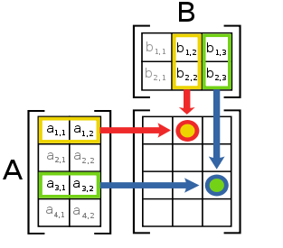
When multiplying two matrices m and n, the resulting matrix will have the same number of rows as m and the same number of columns as n. Each element of the result matrix can be found by taking the dot product of each row of m and each column of n.


When viewed this way, it's easy to see that each row the resulting matrix is the product of a row in the first input matrix (m) and the entire second input matrix (n). Using this knowledge, we can define multiplication of two matrices in terms of matrix-*-vector.

(define (matrix-*-matrix m n)
   (let ((cols (transpose n)))
     (map (lambda (row) (matrix-*-vector cols row)) m)))

Testing

We have to remember a few rules of matrix algebra that aren't enforced in the procedures we've defined.

• For dot-product, two vectors can only be multiplied if they're the same length.
• For matrix-*-vector, the vector must be the same length as the number of columns in the matrix.
• For matrix-*-matrix, two matrices A and B can be multiplied only if the number of columns of A matches the number of rows of B.

> (define v (list 1 3 -5))
> (define w (list 4 -2 -1))
> (dot-product v w)
3
> (define m (list (list 1 2 3) (list 4 5 6)))
> (define v (list 1 2 3))
> (matrix-*-vector m v)
(14 32)
> (define a (list (list 14 9 3) (list 2 11 15) (list 0 12 17) (list 5 2 3)))
> (define b (list (list 12 25) (list 9 10) (list 8 5)))
> (matrix-*-matrix a b)
((273 455) (243 235) (244 205) (102 160))

Note that the values above are the same as those used as as examples on pages I linked to explaining each operation. The results above are correct, but you can do a Google search for "matrix multiplication calculator" to find several online calculators if you want to test with other values.


Related:

For links to all of the SICP lecture notes and exercises that I've done so far, see The SICP Challenge.

SICP 2.35: Counting the Leaves of a Tree

From SICP section 2.2.3 Sequences as Conventional Interfaces

Exercise 2.35 asks us to redefine the count-leaves procedure from section 2.2.2 as an accumulation. Our procedure should take the following form:

(define (count-leaves t)
   (accumulate <??> <??> (map <??> <??>)))

When I encounter a problem like this (implement X in terms of Y), I find that it helps to take a look at both procedures side-by-side to see what they have in common. The count-leaves procedure just returns 1 when it encounters each leaf node, and recursively combines all those 1s with addition otherwise.

; count-leaves from sicp section 2.2.2
(define (count-leaves x)
   (cond ((null? x) 0)
         ((not (pair? x)) 1)
         (else (+ (count-leaves (car x))
                  (count-leaves (cdr x))))))

The accumulate procedure takes an operator, and initial value, and a sequence as its parameters. It then combines all elements of the sequence with the initial value using the operator.

; accumulate from sicp section 2.2.3
(define (accumulate op initial sequence)
   (if (null? sequence)
       initial
       (op (car sequence)
           (accumulate op initial (cdr sequence)))))

The operator and initial value in the case of count-leaves are pretty easy to guess. They should be + and 0 respectively. For its third argument accumulate is expecting a sequence, and our template is using map. Recall that map takes a function and a list and returns a new list. The new list is simply the result of the function being applied to each element of the old list. What we'd really like to accumulate is a sequence of 1s, one for each leaf in the tree. To implement that we need the help of one more procedure from SICP section 2.2.3.

; enumerate-tree from sicp 2.2.3
(define (enumerate-tree tree)
   (cond ((null? tree) null)
         ((not (pair? tree)) (list tree))
        (else (append (enumerate-tree (car tree))
                       (enumerate-tree (cdr tree))))))

The enumerate-tree procedure "flattens out" a tree into a sequence of its leaves. Once we have the tree in the form of a sequence, we just need to define a function for the first argument of map. This function should simply return a 1 for any input. Here's the complete (but very short) solution.

(define (count-leaves t)
   (accumulate + 0 (map (lambda (x) 1)
                        (enumerate-tree t))))

Test it out with trees of different shapes, just to be sure there are no corner cases missed.

> (count-leaves (list))
0
> (count-leaves (list 1 2 3))
3
> (count-leaves (list 1 (list 1 2 3)))
4
> (count-leaves (list (list 1 2) (list 1 2 3) 1))
6

Related:

For links to all of the SICP lecture notes and exercises that I've done so far, see The SICP Challenge.

SICP 2.34: Horner's rule

From SICP section 2.2.3 Sequences as Conventional Interfaces

Exercise 2.34 introduces Horner's rule, an algorithm for the efficient evaluation of polynomial expressions at a given value of x. Horner's rule evaluates a polynomial expression using the fewest possible number of additions and multiplications.

Let's take a look at a specific example to see how this works.

4x³ + 3x² + 2x + 1

The terms of the polynomial above can be grouped as follows

(4x³ + 3x² + 2x) + 1

Once that grouping is in place it's easier to see that you can now factor out an x from the term in parentheses.

x * (4x² + 3x + 2) + 1

Now you can apply the same grouping and factoring steps to the term left in parentheses.

x * (x * (4x + 3) + 2) + 1

This is as far as we can go because another x cannot be factored out of the term in the innermost parentheses.

More generally, Horner's rule says that the polynomial

a_nxⁿ + a_n-1x^n-1 + ... + a₀

can be evaluated as

((a_nx + a_n-1)x + ...)x + a₀

This reduces the total number of multiplications performed because the exponents in each term of the original polynomial are not computed separately.

Using Horner's rule, evaluating polynomials can be formulated as an accumulation. Our task in this exercise is to complete the following implementation, assuming that the coefficients of the polynomial are arranged in a sequence from a₀ through a_n.

(define (horner-eval x coefficient-sequence)
   (accumulate (lambda (this-coeff higher-terms) <??>)
               0
               coefficient-sequence))

Given the framework and assumption above, there really are not a lot of different ways to go about this. The accumulate procedure is already doing most of the work for us, recursively accumulating the terms of the polynomial in the order that they're (conveniently) provided. All we have to do is implement the operator function that gets passed to accumulate.

The piece that we need to implement is summarized in the text as follows:

In other words, we start with a_n, multiply by x, add a_n-1, multiply by x, and so on, until we reach a₀.

In our lambda, a₀ through a_n are represented by this-coeff, so all we need to do is add this-coeff to the accumulation and multiply by x.

(define (horner-eval x coefficient-sequence)
   (accumulate (lambda (this-coeff higher-terms)
                 (+ (* x higher-terms) this-coeff))
               0
               coefficient-sequence))

Here also is the implementation of accumulate so you can test the horner-eval procedure.

(define (accumulate op initial sequence)
   (if (null? sequence)
       initial
       (op (car sequence)
           (accumulate op initial (cdr sequence)))))

Let's start with a simpler test case than the one provided in the text and add terms so we can more easily predict what the correct output should be. The first example below is evaluating the polynomial (1 + 3x) where x = 2, and the final example is evaluating (1 + 3x + 5x³ + x⁵), also at x = 2.

> (horner-eval 2 (list 1 3))
7
> (horner-eval 2 (list 1 3 0))
7
> (horner-eval 2 (list 1 3 0 5))
47
> (horner-eval 2 (list 1 3 0 5 0))
47
> (horner-eval 2 (list 1 3 0 5 0 1))
79

Related:

For an interesting application of Horner's rule, see the solution to Look And Say, Revisited from Programming Praxis.

For links to all of the SICP lecture notes and exercises that I've done so far, see The SICP Challenge.