SICP 2.38 & 2.39: Folding Left and Right

From SICP section 2.2.3 Sequences as Conventional Interfaces

Exercise 2.38 informs us that another name for the accumulate procedure we've been using is fold-right, because it combines the elements of a sequence starting on the left and moving to the right. There's also a fold-left procedure that combines elements working in the opposite direction.

; fold-right is another name for accumulate
(define (fold-right op initial sequence)
   (if (null? sequence)
       initial
       (op (car sequence)
           (fold-right op initial (cdr sequence)))))

; fold-left is given in exercise 2.38
(define (fold-left op initial sequence)
   (define (iter result rest)
     (if (null? rest)
         result
         (iter (op result (car rest))
               (cdr rest))))
   (iter initial sequence))

We're given a few expressions that illustrate how these two procedures behave differently.

> (fold-right / 1 (list 1 2 3))
1 1/2
> (fold-left / 1 (list 1 2 3))
1/6
> (fold-right list null (list 1 2 3))
(1 (2 (3 ())))
> (fold-left list null (list 1 2 3))
(((() 1) 2) 3)

We're asked what property the op parameter needs to satisfy to guarantee that fold-right and fold-left will produce the same values for any sequence.

The property that will guarantee that fold-right and fold-left will produce the same values for any sequence is commutativity. You may remember the commutative property of both addition and multiplication from algebra. It's the law that says that:

A + B = B + A

and

A x B = B x A

Subtraction and division are not commutative operations. The AND and OR operations in Boolean algebra are commutative.


Exercise 2.39 asks us to complete the following definitions of reverse (from exercise 2.18) in terms of fold-right and fold-left:

(define (reverse sequence)
   (fold-right (lambda (x y) <??>) null sequence))

(define (reverse sequence)
   (fold-left (lambda (x y) <??>) null sequence))

Since we only need to define the operator used in each implementation, the key to this exercise lies in how the operator is applied in each folding procedure. Pay close attention to the order of the arguments of the op procedure.

In fold-right the operator is applied to the car of the sequence and the result of a recursive call to fold-right. Just as we did in exercise 2.18, we can reverse the sequence using fold-right by appending the car of the sequence to the reverse of its cdr.

(define (reverse sequence)
   (fold-right (lambda (x y) (append y (list x))) null sequence))

In fold-left the operator is applied to the result sequence and the car of the unused elements in the initial sequence. Since the result sequence starts with an initial value of null, and we're starting at the end of the sequence and working backwards anyway, we can just cons each element to the end of the result.

(define (reverse sequence)
   (fold-left (lambda (x y) (cons y x)) null sequence))

As expected, we get the same test results for either of the two reverse implementations above.

> (reverse (list 1 2 3 4))
(4 3 2 1)
> (reverse (list 1 4 9 16 25))
(25 16 9 4 1)
> (reverse (list 1 3 5 7))
(7 5 3 1)
> (reverse (list 23 72 149 34))
(34 149 72 23)

Related:

For links to all of the SICP lecture notes and exercises that I've done so far, see The SICP Challenge.

SICP 2.36 & 2.37: Matrix Algebra

From SICP section 2.2.3 Sequences as Conventional Interfaces

Exercise 2.36 asks us to complete the accumulate-n procedure, which is similar to accumulate except that it takes as its third argument a sequence of sequences that are assumed to all have the same length. It applies the accumulation procedure to all the first elements of the sub-sequences, all the second elements, third elements, and so on and returns a sequence of the results. For example, given the sequence s containing the following values, ((1 2 3) (4 5 6) (7 8 9) (10 11 12)), the value of (accumulate-n + 0 s) should return the sequence (22 26 30).

Our task is to fill in the missing expressions in the following definition:

(define (accumulate-n op init seqs)
   (if (null? (car seqs))
       null
       (cons (accumulate op init <??>)
             (accumulate-n op init <??>))))

If you've been doing all the exercises up to this point, then this procedure's overall structure of recursively building up a sequence with cons will be familiar.

In exercise 2.35 we used map and a simple lambda expression to flatten out a tree so the result could be used as the third parameter to accumulate. We can do something very similar here to fill in the missing expressions above. We'll still use map to loop over each of the sub-sequences, but in this case we need map to return a sequence that contains the first element from each sub-sequence (in the first missing expression) and the remaining elements of each sub-sequence (in the second missing expression). We already know two procedures that meet those needs, car and cdr.

; accumulate from sicp section 2.2.3
(define (accumulate op initial sequence)
   (if (null? sequence)
       initial
       (op (car sequence)
           (accumulate op initial (cdr sequence)))))

(define (accumulate-n op init seqs)
   (if (null? (car seqs))
       null
       (cons (accumulate op init (map car seqs))
             (accumulate-n op init (map cdr seqs)))))

The first call to map returns a sequence containing the first element of each of the original sub-sequences. The second call to map returns the sequence of sub-sequences with each of their first elements removed. This continues recursively until no more elements remain. We can test the solution with the values given in the exercise.

> (define s (list (list 1 2 3) (list 4 5 6) (list 7 8 9) (list 10 11 12)))
> s
((1 2 3) (4 5 6) (7 8 9) (10 11 12))
> (accumulate-n + 0 s)
(22 26 30)

Exercise 2.37 introduces a representation for vectors and matrices. A vector can be represented as a sequence of numbers, and a matrix as a sequence of vectors. For example, the matrix


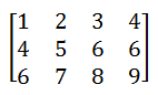
can be represented as the sequence ((1 2 3 4) (4 5 6 6) (6 7 8 9)).

We can use this representation to express the basic operations of matrix algebra in terms of sequence operations. These basic operations are:

(dot-product v w) - returns the sum Σ_i(v_iw_i)

(matrix-*-vector m v) - returns the vector t, where t_i = Σ_j(m_ijv_j)

(matrix-*-matrix m n) - returns the matrix p, where p_ij = Σ_k(m_ikn_kj)

(transpose mat) - returns the matrix n, where n_ij = m_ji


Dot product

The dot product is defined for us.

(define (dot-product v w)
   (accumulate + 0 (map * v w)))

The dot-product procedure takes two vectors (that are assumed to be equal length) and returns a single number obtained by multiplying corresponding elements and then summing those products.

Note that the use of map in this procedure takes more arguments than we've seen up to this point. That's because map takes a procedure of n arguments, together with n lists, and applies the procedure to all the first elements of the lists, all the second elements of the lists, and so on, returning a list of the results. Up to this point, we've been using map where n = 1.

Our task is to fill in the missing expressions in the given procedures for computing the remaining matrix operations. Let's take them one at a time.


Multiply a matrix by a vector

(define (matrix-*-vector m v)
   (map <??> m))

When multiplying a matrix by a vector, each row of the matrix is multiplied by the vector (using the dot product procedure described above). The result is a vector containing each dot product. Since map will pass each row of the matrix to whatever function we provide, we can just define a lambda expression that uses the dot-product procedure already defined.

(define (matrix-*-vector m v)
   (map (lambda (row) (dot-product row v)) m))

Transpose a matrix

(define (transpose mat)
   (accumulate-n <??> <??> mat))

There are several ways of looking at matrix transposition, but the one that makes the most sense given the code above is to write the columns of the input matrix as the rows of the output matrix. Remember that accumulate-n will combine the columns with whatever function we give it, and this part of the exercise is a snap.

(define (transpose mat)
   (accumulate-n cons null mat))

We can test this procedure with the matrix s defined in the exercise above.

> (define s (list (list 1 2 3) (list 4 5 6) (list 7 8 9) (list 10 11 12)))
> (transpose s)
((1 4 7 10) (2 5 8 11) (3 6 9 12))

Multiply two matrices

(define (matrix-*-matrix m n)
   (let ((cols (transpose n)))
      (map <??> m)))

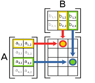
When multiplying two matrices m and n, the resulting matrix will have the same number of rows as m and the same number of columns as n. Each element of the result matrix can be found by taking the dot product of each row of m and each column of n.


When viewed this way, it's easy to see that each row the resulting matrix is the product of a row in the first input matrix (m) and the entire second input matrix (n). Using this knowledge, we can define multiplication of two matrices in terms of matrix-*-vector.

(define (matrix-*-matrix m n)
   (let ((cols (transpose n)))
     (map (lambda (row) (matrix-*-vector cols row)) m)))

Testing

We have to remember a few rules of matrix algebra that aren't enforced in the procedures we've defined.

• For dot-product, two vectors can only be multiplied if they're the same length.
• For matrix-*-vector, the vector must be the same length as the number of columns in the matrix.
• For matrix-*-matrix, two matrices A and B can be multiplied only if the number of columns of A matches the number of rows of B.

> (define v (list 1 3 -5))
> (define w (list 4 -2 -1))
> (dot-product v w)
3
> (define m (list (list 1 2 3) (list 4 5 6)))
> (define v (list 1 2 3))
> (matrix-*-vector m v)
(14 32)
> (define a (list (list 14 9 3) (list 2 11 15) (list 0 12 17) (list 5 2 3)))
> (define b (list (list 12 25) (list 9 10) (list 8 5)))
> (matrix-*-matrix a b)
((273 455) (243 235) (244 205) (102 160))

Note that the values above are the same as those used as as examples on pages I linked to explaining each operation. The results above are correct, but you can do a Google search for "matrix multiplication calculator" to find several online calculators if you want to test with other values.


Related:

For links to all of the SICP lecture notes and exercises that I've done so far, see The SICP Challenge.

SICP 2.35: Counting the Leaves of a Tree

From SICP section 2.2.3 Sequences as Conventional Interfaces

Exercise 2.35 asks us to redefine the count-leaves procedure from section 2.2.2 as an accumulation. Our procedure should take the following form:

(define (count-leaves t)
   (accumulate <??> <??> (map <??> <??>)))

When I encounter a problem like this (implement X in terms of Y), I find that it helps to take a look at both procedures side-by-side to see what they have in common. The count-leaves procedure just returns 1 when it encounters each leaf node, and recursively combines all those 1s with addition otherwise.

; count-leaves from sicp section 2.2.2
(define (count-leaves x)
   (cond ((null? x) 0)
         ((not (pair? x)) 1)
         (else (+ (count-leaves (car x))
                  (count-leaves (cdr x))))))

The accumulate procedure takes an operator, and initial value, and a sequence as its parameters. It then combines all elements of the sequence with the initial value using the operator.

; accumulate from sicp section 2.2.3
(define (accumulate op initial sequence)
   (if (null? sequence)
       initial
       (op (car sequence)
           (accumulate op initial (cdr sequence)))))

The operator and initial value in the case of count-leaves are pretty easy to guess. They should be + and 0 respectively. For its third argument accumulate is expecting a sequence, and our template is using map. Recall that map takes a function and a list and returns a new list. The new list is simply the result of the function being applied to each element of the old list. What we'd really like to accumulate is a sequence of 1s, one for each leaf in the tree. To implement that we need the help of one more procedure from SICP section 2.2.3.

; enumerate-tree from sicp 2.2.3
(define (enumerate-tree tree)
   (cond ((null? tree) null)
         ((not (pair? tree)) (list tree))
        (else (append (enumerate-tree (car tree))
                       (enumerate-tree (cdr tree))))))

The enumerate-tree procedure "flattens out" a tree into a sequence of its leaves. Once we have the tree in the form of a sequence, we just need to define a function for the first argument of map. This function should simply return a 1 for any input. Here's the complete (but very short) solution.

(define (count-leaves t)
   (accumulate + 0 (map (lambda (x) 1)
                        (enumerate-tree t))))

Test it out with trees of different shapes, just to be sure there are no corner cases missed.

> (count-leaves (list))
0
> (count-leaves (list 1 2 3))
3
> (count-leaves (list 1 (list 1 2 3)))
4
> (count-leaves (list (list 1 2) (list 1 2 3) 1))
6

Related:

For links to all of the SICP lecture notes and exercises that I've done so far, see The SICP Challenge.

SICP 2.34: Horner's rule

From SICP section 2.2.3 Sequences as Conventional Interfaces

Exercise 2.34 introduces Horner's rule, an algorithm for the efficient evaluation of polynomial expressions at a given value of x. Horner's rule evaluates a polynomial expression using the fewest possible number of additions and multiplications.

Let's take a look at a specific example to see how this works.

4x³ + 3x² + 2x + 1

The terms of the polynomial above can be grouped as follows

(4x³ + 3x² + 2x) + 1

Once that grouping is in place it's easier to see that you can now factor out an x from the term in parentheses.

x * (4x² + 3x + 2) + 1

Now you can apply the same grouping and factoring steps to the term left in parentheses.

x * (x * (4x + 3) + 2) + 1

This is as far as we can go because another x cannot be factored out of the term in the innermost parentheses.

More generally, Horner's rule says that the polynomial

a_nxⁿ + a_n-1x^n-1 + ... + a₀

can be evaluated as

((a_nx + a_n-1)x + ...)x + a₀

This reduces the total number of multiplications performed because the exponents in each term of the original polynomial are not computed separately.

Using Horner's rule, evaluating polynomials can be formulated as an accumulation. Our task in this exercise is to complete the following implementation, assuming that the coefficients of the polynomial are arranged in a sequence from a₀ through a_n.

(define (horner-eval x coefficient-sequence)
   (accumulate (lambda (this-coeff higher-terms) <??>)
               0
               coefficient-sequence))

Given the framework and assumption above, there really are not a lot of different ways to go about this. The accumulate procedure is already doing most of the work for us, recursively accumulating the terms of the polynomial in the order that they're (conveniently) provided. All we have to do is implement the operator function that gets passed to accumulate.

The piece that we need to implement is summarized in the text as follows:

In other words, we start with a_n, multiply by x, add a_n-1, multiply by x, and so on, until we reach a₀.

In our lambda, a₀ through a_n are represented by this-coeff, so all we need to do is add this-coeff to the accumulation and multiply by x.

(define (horner-eval x coefficient-sequence)
   (accumulate (lambda (this-coeff higher-terms)
                 (+ (* x higher-terms) this-coeff))
               0
               coefficient-sequence))

Here also is the implementation of accumulate so you can test the horner-eval procedure.

(define (accumulate op initial sequence)
   (if (null? sequence)
       initial
       (op (car sequence)
           (accumulate op initial (cdr sequence)))))

Let's start with a simpler test case than the one provided in the text and add terms so we can more easily predict what the correct output should be. The first example below is evaluating the polynomial (1 + 3x) where x = 2, and the final example is evaluating (1 + 3x + 5x³ + x⁵), also at x = 2.

> (horner-eval 2 (list 1 3))
7
> (horner-eval 2 (list 1 3 0))
7
> (horner-eval 2 (list 1 3 0 5))
47
> (horner-eval 2 (list 1 3 0 5 0))
47
> (horner-eval 2 (list 1 3 0 5 0 1))
79

Related:

For an interesting application of Horner's rule, see the solution to Look And Say, Revisited from Programming Praxis.

For links to all of the SICP lecture notes and exercises that I've done so far, see The SICP Challenge.