SICP Exercise 1.30: Iterative Sums

From SICP section 1.3.1 Procedures as Arguments

Exercise 1.30 asks us to transform the now familiar recursive sum procedure (see exercise 1.29) into an iterative one. We're given the following template to get us started:

(define (sum term a next b)
 (define (iter a result)
   (if <??>
       <??>
       (iter <??> <??>)))
 (iter <??> <??>))

If you need a refresher on recursive and iterative processes, take a look back at SICP section 1.2.1 Linear Recursion and Iteration. The iterative factorial example given in that section has a lot in common with our template:

(define (factorial n)
 (fact-iter 1 1 n))

(define (fact-iter product counter max-count)
 (if (> counter max-count)
     product
     (fact-iter (* counter product)
                (+ counter 1)
                max-count)))

The key to this procedure is the use of state variables, particularly product, which holds the result of multiplying all the values from 1 to n as the process moves from state to state. In our iterative sum procedure, result will serve as the same kind of state variable, storing the sum of all the terms.

The first two pieces are pretty easy to get. If a is greater than b, we just want to return the result.

(define (sum term a next b)
 (define (iter a result)
   (if (> a b)
       result
       (iter <??> <??>)))
 (iter <??> <??>))

The next two pieces are the really interesting parts. These are our state variables that make the iterative process work. We need to decide what values to store in a and result for the next iteration to work with. The value passed in for a should be the next term in the series, and the value passed in for result should just add the current term to the result.

(define (sum term a next b)
 (define (iter a result)
   (if (> a b)
       result
       (iter (next a) (+ (term a) result))))
 (iter <??> <??>))

Finally, we just need to define the starting values for the iterative process. The starting value for a should just be the same a passed in to the sum procedure, and since we're accumulating a sum, the starting value for result should be 0.

(define (sum term a next b)
 (define (iter a result)
   (if (> a b)
       result
       (iter (next a) (+ (term a) result))))
 (iter a 0))

If you substitute this procedure in for the old one that we used in exercise 1.29, you should see that you get the same results.


Related:

For links to all of the SICP lecture notes and exercises that I've done so far, see The SICP Challenge.

SICP Exercise 1.29: Integration using Simpson's Rule

From SICP section 1.3.1 Procedures as Arguments

Exercise 1.29 asks us to define a procedure that uses Simpson's rule to approximate the value of the integral of a function between two values. (Informally, you may remember that the integral of a function is the area under the curve of that function.)

We're given a big head start earlier in the section when an integral procedure is defined using a different method.

(define (sum term a next b)
  (if (> a b)
      0
      (+ (term a)
         (sum term (next a) next b))))

(define (integral f a b dx)
  (define (add-dx x) (+ x dx))
  (* (sum f (+ a (/ dx 2.0)) add-dx b)
     dx))

We're told to use this procedure to check our results by integrating cube between 0 and 1.

Simpson's rule states that the integral of a function f between a and b is approximated as

h(y₀ + 4y₁ + 2y₂ + 4y₃ + 2y₄ + ... + 2y_n-2 + 4y_n-1 + y_n) / 3

where h = (b - a)/n, for some even integer n, and y_k = f(a + kh).

This is the sum of a series, so we'll still be defining our new procedure in terms of the sum procedure used before. Using Simpson's rule, the sum of a series is multiplied by h and divided by 3, so we'll start with that and a little of the "wishful thinking" that Professor Abelson spoke so highly of in lecture 2A.

(define (simpson f a b n)
   (/ (* h (sum term 0 inc n)) 3))

Now that we know how Simpson's rule can be defined in terms of sum, we just need to fill in the pieces that are missing.

The variable h is pretty easy to define from the description.

(define h (/ (- b a) n))

The procedure used to get from one term of the series to the next is even simpler. n is just incremented by one at each step, so we just need to define a procedure to do that.

(define (inc x) (+ x 1))

We know that the sum procedure takes two functions, term and next, and two values a and b, and computes the sum of the terms of the function from a to b. Defining the terms of the series in Simpson's rule is a two-step process. First we have to define the function for computing y_k, which is given.

(define (y k)
   (f (+ a (* k h))))

Next we have to define a rule for computing the coefficient for each of the k terms. Once we know the coefficient we'll just multiply it by y_k to get the complete term. The rules for defining the coefficients are pretty simple. Notice that if k is odd, then the coefficient is always 4. If k is even, then the coefficient is usually 2, except for the first (0th) and last (nth) terms, where the coefficient is 1.

(define (term k)
   (* (cond ((odd? k) 4)
            ((or (= k 0) (= k n)) 1)
            ((even? k) 2))
      (y k)))

Putting this all together, we have the complete procedure:

(define (simpson f a b n)
  (define h (/ (- b a) n))
  (define (inc x) (+ x 1))
  (define (y k)
    (f (+ a (* k h))))
  (define (term k)
    (* (cond ((odd? k) 4)
             ((or (= k 0) (= k n)) 1)
             ((even? k) 2))
       (y k)))
  (/ (* h (sum term 0 inc n)) 3))

The only thing left to do is to define a cube procedure and compare the results of simpson with those of the old integral procedure that we were given.

(define (cube x) (* x x x))

> (integral cube 0 1 0.01)
0.24998750000000042
> (simpson cube 0 1 100.0)
0.24999999999999992
> (integral cube 0 1 0.001)
0.249999875000001
> (simpson cube 0 1 1000.0)
0.2500000000000003

As you can see from these results, Simpson's rule gives us a much better approximation to the integral when computing the same number of terms.


Related:

For links to all of the SICP lecture notes and exercises that I've done so far, see The SICP Challenge.

SICP Lecture 2A: Higher-order Procedures

Structure and Interpretation of Computer Programs
Higher-order Procedures
Covers Text Section 1.3

You can download the video lecture or stream it on MIT's OpenCourseWare site. It's also available on YouTube.

This lecture is presented by MIT's Professor Gerald Jay Sussman.

Introduction

So far in the SICP lectures and exercises, we've seen that we can use procedures to describe compound operations on numbers. This is a first-order abstraction. Instead of performing primitive operations on the values to solve a distinct instance of a problem, we can write a procedure that performs the correct operations, then tell it what numbers to operate on when we need it. For example, instead of writing (* 5 5) when we want to find the value of 5 squared, we can define the square procedure:

(define (square x) (* x x))

then just invoke it on any number we need to square.

In this section we'll start to think about higher-order procedures. Instead of simply manipulating data (or more precisely, what we are used to thinking of as data), as in the procedures we've written so far, higher-order procedures manipulate other procedures by accepting them as arguments or returning them as values.

Procedures as Arguments

The video lecture explains this concept by looking at three very similar procedures, then showing how one idea can be refactored out of them to create a procedure that can be reused. The three procedures are the sum of the integers from a to b, the sum of the squares from a to b (the text book uses the sum of cubes), and Leibniz's formula for finding π/8.

(define (sum-int a b)
 (if (> a b)
     0
     (+ a (sum-int (+ a 1) b))))

(define (sum-sq a b)
  (if (> a b)
      0
      (+ (square a) (sum-sq (+ a 1) b))))

(define (pi-sum a b)
  (if (> a b)
      0
      (+ (/ 1.0 (* a (+ a 2)))
         (pi-sum (+ a 4) b))))

As you can see, these procedures are all nearly identical. The only things that are different are the function being applied to each term in the sequence, how you get to the next term of the sequence, and the names of the procedures themselves. We can use the similarities of these procedures to create a general pattern that describes all three.

(define (<name> a b)
  (if (> a b)
      0
      (+ <term> (<name> (<next> a) b))))

The general pattern is that the procedure:

• is given a name
• takes two arguments (a lower bound and an upper bound)
• performs a test to see if the upper bound is exceeded
• applies some procedure to the current term and adds the result to the recursive call to get the next term
• computes of the next term

The important thing to note here is that some of the things that change are procedures, not just numbers.

There's nothing very special about numbers. Numbers are just one kind of data.

Since procedures are also a type of data in Scheme, we can use them as arguments to other procedures as well. Now that we have a general pattern, we use it to define a sigma procedure.

(define (sum term a next b)
  (if (> a b)
      0
      (+ (term a)
         (sum term (next a) next b))))

The arguments term and next are procedures that are passed in to the sum procedure, and will be used to compute the value of the current term and how to get to the next one.

We can use the procedure above to rewrite sum-int as follows:

(define (sum-int a b)
  (define (identity x) x)
  (sum identity a inc b))

First, the identity procedure simply takes an argument and returns that argument. We need this because the sum-int procedure doesn't apply any function to each term of the sequence, it just sums up the raw terms. Our sum procedure is expecting a procedure as its second argument, so we have to give it one. Next we simply call the sum procedure, passing in the identity and increment procedures for term and next.

The sum-sq and pi-sum procedures can be rewritten as well (which is kind of the point).

(define (sum-sq a b)
  (define (identity x) x)
  (sum square a inc b))

(define (pi-sum a b)
  (sum (lambda (i) (/ 1.0 (* x (+ x 2))))
       a
       (lambda (i) (+ x 4))
       b))

Note that in the pi-sum example, we use lambda notation to define the procedures for term and next as we are passing them in to sum. We can redefine pi-sum without lambda notation by explicitly defining named procedures.

(define (pi-sum a b)
  (define (pi-term x)
     (/ 1.0 (* x (+ x 2))))
  (define (pi-next x)
     (+ x 4))
  (sum pi-term a pi-next b))

This makes no difference in how the code is evaluated. In the first example we passed a procedure by its definition, in the second we passed it by its name. In future articles on lectures and exercises, I'll be using more and more lambda notation since we should be becoming more familiar with it.

Separating the abstract idea of sum into its own procedure allows us to reuse it in several situations where that idea is needed. Another important point is that we could reimplement sum itself, in perhaps a more efficient way, and we would benefit from it everywhere it is used without having to rewrite all the procedures that use it. Here's an iterative implementation of sum.

(define (sum term a next)
  (define (iter j ans)
      (if (> j b)
          ans
          (iter (next j)
                (+ (term j) ans))))
  (iter a 0))

Decomposing procedures in this way allows us to change one abstraction without needing to change the every procedure where it is used. If we wanted to use the iterative approach to summation in the original three procedures at the top, we'd have to rewrite all three of them individually. Putting the summation code in its own procedure allows you to change it in one place, but use it everywhere the procedure is called.


Abstraction

In section 1.1.8 we looked at Heron of Alexandria's method for computing a square root.

(define (sqrt x)
  (define tolerance 0.00001)
  (define (good-enough? y)
     (< (abs (- (* y y) x)) tolerance ))
  (define (improve y)
     (average (/ x y) y))
  (define (try y)
     (if (good-enough? y)
         y
        (try (improve y))))
  (try 1))

The algorithm for computing the square root of x is not intuitively obvious from looking at the code in this procedure. In this section we'll show how abstraction can be used to clarify how this procedure works.

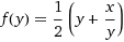
The procedure iteratively improves a guess until it is within a pre-defined tolerance of the correct answer. The function for improving the guess for the square root of x is to average the guess with x divided by x. In mathematical terms


If you substitute in √x for y, you'll notice that we're looking for a fixed point of this function. (A fixed point of a function is a point that is mapped to itself by the function. If you put a fixed point into a function, you get the same value out.)

f(y) = (y + x/y) / 2
f(√x) = (√x + x/√x) / 2
f(√x) = (√x + √x) / 2
f(√x) = 2 * √x / 2
f(√x) = √x

We can use this to rewrite the sqrt procedure in terms of computing a fixed point. (Even though we don't have a procedure to compute a fixed point yet. That will be coming up next.)

(define (sqrt x)
  (fixed-point
      (lambda (y) (average (/ x y) y))
      1))

This procedure shows how to compute the square root of x in terms of computing a fixed point, but from this we only know that what we pass to the fixed-point procedure is another procedure and an initial guess. At this point, fixed-point is only "wishful thinking." Here's one way to compute fixed points of a function:

(define (fixed-point f start)
  (define tolerance 0.00001)
  (define (close-enuf? u v)
     (< (abs (- u v)) tolerance))
  (define (iter old new)
     (if (close-enuf? old new)
         new
         (iter new (f new))))
  (iter start (f start)))

This procedure computes:

the fixed point of the function computed by the procedure whose name will be "f" in this procedure.

This is a key quote from the lecture because it illustrates how procedures can treated like any other data in Scheme. Here, the variable f can take on the value of any procedure you want to pass in.

The fixed point of the function passed in to fixed-point is computed by iteratively applying the function to its own result, starting at the initial guess, until the change in the result is smaller than some tolerance. Note how the function that is passed in as the parameter f is evaluated in the iteration loop.

If you define an average procedure you can run the new sqrt procedure in a Scheme interpreter to test it out.

(define (average x y)
  (/ (+ x y) 2))

Procedures as Returned Values

There's another abstraction that we can pull out of the previous fixed-point procedure. Before we get to that, a simpler procedure for computing functions whose fixed point is the square root is:

g(y) = x/y

This has the same property as the function we looked at before, if you insert √x in for y, you get √x back. The reason that we didn't use this simpler function before is that for some inputs it will oscillate. If x is 2, and your initial guess is 1, then the old and new values will oscillate between 2 and 1, never getting any closer together. The original function that uses the average procedure is just damping out this oscillation. We can pull this damping concept out by first defining sqrt as a function of a fixed-point procedure that is itself a function of average damping.

(define (sqrt x)
  (fixed-point
      (average-damp (lambda (y) (/ x y)))
      1))

Here, average-damp takes a procedure as its argument and returns a procedure as its value. When given a procedure that takes an argument, average-damp returns another procedure that computes the average of the values before and after applying the original procedure to its argument.

(define average-damp
  (lambda (f)
      (lambda (x) (average (f x) x))))

This is special because it's the first time we've seen a procedure that produces a procedure as its result.


Newton's method

A general method for finding roots (zeroes) of functions is called Newton's method. To find a y such that

f(y) = 0

the general procedure is to start with a guess y₀, then iterate the following expression using the function:

y_n+1 = y_n - f(y_n) / df/dy | y = y_n

This is a difference equation. Each term is the difference between the previous term and the function applied to the previous term divided by the derivative with respect to y of f evaluated at the previous term. (The Scheme representation of this should be a lot more clear, but for now we just need to remember that the derivative of f with respect to y is a function.) We'll start the same way we did before, by applying the method before we define it.

We can define sqrt in terms of Newton's method as follows:

(define (sqrt x)
  (newton (lambda (y) (- x (square y)))
          1))

The square root of x is computed by applying Newton's method to the function of y that computes the difference between x and the square of y. If we had a value of y for which the difference between x and y² returned 0, then y would be the square root of x.

Now we have to define a procedure for Newton's method. Note that we're still using a method of iteratively improving a guess, just as we did in the earlier sqrt procedures. Look again at the expression for Newton's method:

y_n+1 = y_n - f(y_n) / df/dy | y = y_n

We'd like to find some value for y_n such that when we plug it in on the right hand side of this expression, we get the same value back out on the left hand side (within some small tolerance). So once again, we are looking for a fixed point.

(define (newton f guess)
  (define df (deriv f))
  (fixed-point
      (lambda (x) (- x (/ (f x) (df x))))
      guess))

This procedure takes a function and an initial guess, and computes the fixed point of the function that computes the difference of x and the quotient of the function of x and the derivative of the function of x.

Wishful thinking is essential to good engineering, and certainly essential to good computer science.

Along the way we have to write a procedure that computes the derivative (a function) of the function passed to it.

(define deriv
  (lambda (f)
      (lambda (x)
          (/ (- (f (+ x dx))
             (f x))
          dx))))

(define dx 0.0000001)

You may remember from Calculus or a past life that the derivative of a function is the function of x that computes

f(x + Δx) - f(x) / Δx

for some small value of Δx. You might also remember (and perhaps a bit more readily) that the derivative of x² is 2x. So if we apply our deriv procedure to square, we should expect to get back a procedure that computes 2x. Unfortunately when I tried it in a Scheme interpreter I got back:

> (deriv square)
#<procedure>

That's not very revealing, so we're not done experimenting yet. How can we figure out what that returned procedure does? Let's just apply it to some values.

> ((deriv square) 2)
4.000000091153311
> ((deriv square) 5)
10.000000116860974
> ((deriv square) 10)
19.999999949504854
> ((deriv square) 25)
50.00000101063051
> ((deriv square) 100)
199.99999494757503

That looks like a fair approximation to the expected procedure.


Abstractions and first-class procedures

The lecture wraps up with the following list by computer scientist Christopher Strachey, one of the inventors of denotational semantics.

The rights and privileges of first-class citizens:

• To be named by variables.
• To be passed as arguments to procedures.
• To be returned as values of procedures.
• To be incorporated into data structures.

We've seen that both values and procedures in Scheme meet the first three requirements. In later sections we'll see that they both meet the fourth requirement as well.

Having procedures as first class data allows us to make powerful abstractions that encode general methods like Newton's method in a very clear way.

For links to all of the SICP lecture notes and exercises that I've done so far, see The SICP Challenge.