Showing posts with label sicp. Show all posts

Tuesday, April 30, 2013

SICP 2.66: Sets and information retrieval

From SICP section 2.3.3 Sets and information retrieval

The final part of section 2.3.3 asks us to consider a database that contains records, each of which has a key and some data. If the database is represented as an unordered list, a record can be looked up by its key using the following procedure.

(define (lookup given-key set-of-records)
  (cond ((null? set-of-records) false)
        ((equal? given-key (key (car set-of-records)))
         (car set-of-records))
        (else (lookup given-key (cdr set-of-records)))))

We can define simple procedures for making a record out of a key and its data, and for extracting the key and data from an existing record in order to test the procedure above.

(define (key record) (car record))
(define (data record) (cdr record))
(define (make-record key data) (cons key data))

(define database
  (list (make-record 1 'Bill)
        (make-record 2 'Joe)
        (make-record 3 'Frank)
        (make-record 4 'John)))
  
> (lookup 3 database)
'(3 . Frank)
> (data (lookup 1 database))
'Bill

Exercise 2.66 asks us to implement the lookup procedure for the case where the set of records is structured as a binary tree, ordered by the numerical values of the keys.

We can start by including the list->tree and partial-tree procedures given for exercise 2.64, along with a few required supporting procedures.

(define (entry tree) (car tree))
(define (left-branch tree) (cadr tree))
(define (right-branch tree) (caddr tree))
(define (make-tree entry left right)
  (list entry left right))
  
(define (list->tree elements)
  (car (partial-tree elements (length elements))))

(define (partial-tree elts n)
  (if (= n 0)
      (cons '() elts)
      (let ((left-size (quotient (- n 1) 2)))
        (let ((left-result (partial-tree elts left-size)))
          (let ((left-tree (car left-result))
                (non-left-elts (cdr left-result))
                (right-size (- n (+ left-size 1))))
            (let ((this-entry (car non-left-elts))
                  (right-result (partial-tree (cdr non-left-elts)
                                              right-size)))
              (let ((right-tree (car right-result))
                    (remaining-elts (cdr right-result)))
                (cons (make-tree this-entry left-tree right-tree)
                      remaining-elts))))))))

This makes it easier to convert the existing database to one structured as a binary tree.

> (define tree-db (list->tree database))
> tree-db
'((2 . Joe) ((1 . Bill) () ()) ((3 . Frank) () ((4 . John) () ())))

Finally, we can write the new implementation of lookup using element-of-set? as a guide.

(define (lookup given-key set-of-records)
  (cond ((null? set-of-records) #f)
        ((= given-key (key (car set-of-records)))
         (car set-of-records))
        ((< given-key (key (car set-of-records)))
         (lookup given-key (left-branch set-of-records)))
        ((> given-key (key (car set-of-records)))
         (lookup given-key (right-branch set-of-records)))))

> (lookup 3 tree-db)
'(3 . Frank)
> (lookup 1 tree-db)
'(1 . Bill)
> (lookup 5 tree-db)
#f
> (data (lookup 2 tree-db))
'Joe

For links to all of the SICP lecture notes and exercises that I've done so far, see The SICP Challenge.

Sunday, March 24, 2013

SICP 2.63 - 2.65: Sets as binary trees

From SICP section 2.3.3 Example: Representing Sets

So far in this section we've looked at two ways of representing sets. First as unordered lists, then as ordered lists. Now we'll look at how we can represent sets as binary trees, and we'll see what advantages this representation has over ordered lists.

Each node of a tree holds one element of the set, called the "entry" at that node, and a link to each of two other (possibly empty) nodes. The "left" link points to elements smaller than the one at the node, and the "right" link to elements greater than the one at the node. The same set may be represented by a number of different trees. The only requirements for a valid representation is that all elements in the left subtree must be smaller than the node entry and all elements in the right subtree be must be larger than the node entry. Figure 2.16 in the text shows several valid tree representations of the same set of values.


Recall that for an ordered set of n elements, we had to search through (on average) n/2 elements to locate a particular value. We do this by searching through the elements in order. The advantage of a tree representation is that we can cut this effort down to log n if the tree is balanced.


Exercise 2.63 asks us if the following two procedures produce the same results for every tree, and if not how they differ.

(define (tree->list-1 tree)
  (if (null? tree)
      '()
      (append (tree->list-1 (left-branch tree))
              (cons (entry tree)
                    (tree->list-1 (right-branch tree))))))
     
(define (tree->list-2 tree)
  (define (copy-to-list tree result-list)
    (if (null? tree)
        result-list
        (copy-to-list (left-branch tree)
                      (cons (entry tree)
                            (copy-to-list (right-branch tree)
                                          result-list)))))
  (copy-to-list tree '()))

The tree->list-1 procedure checks to see if the tree passed in is null, and if so returns an empty list. If the tree is not null, it creates a list by appending the left branch of the tree, the element at the root node, and the right branch of the tree. Elements of the left and right branches are flattened into lists using recursive calls to tree->list-1. The tree->list-2 procedure defines a helper function copy-to-list that takes the tree and a result-list as arguments. When the tree is null, it returns the result-list that was passed in. The copy-to-list helper function also uses recursive calls to the left and right branches of the tree while building the final result list. These two procedures will produce the same results for every tree.

We're asked to test the two procedures on the trees in figure 2.16.

(define tree1 '(7 (3 (1 () ()) (5 () ())) (9 () (11 () ()))))
(define tree2 '(3 (1 () ()) (7 (5 () ()) (9 () (11 () ())))))
(define tree3 '(5 (3 (1 () ()) ()) (9 (7 () ()) (11 () ()))))

> (tree->list-1 tree1)
'(1 3 5 7 9 11)
> (tree->list-2 tree1)
'(1 3 5 7 9 11)
> (tree->list-1 tree2)
'(1 3 5 7 9 11)
> (tree->list-2 tree2)
'(1 3 5 7 9 11)
> (tree->list-1 tree3)
'(1 3 5 7 9 11)
> (tree->list-2 tree3)
'(1 3 5 7 9 11)

We can see from these results that both procedures return an in-order traversal for every tree.

We're also asked if the two procedures have the same order of growth for a balanced tree, and if not, which one grows more slowly?

We can see from the results above and from inspecting the two procedures that each node of the tree is visited one time by each algorithm. What happens at each of those n steps is subtly different though. The second procedure simply calls cons at each step, which we'll assume is a constant-time operation, so the tree->list-2 procedure has a time complexity of $O(n)$. The first procedure calls append at each step, which we saw in section 2.2.1 has the following definition:

(define (append list1 list2)
  (if (null? list1)
      list2
      (cons (car list1) (append (cdr list1) list2))))

From this definition we can see that the order of growth of append is proportional to the first list argument that's passed in. In the case of tree->list-1, the first list argument is the left branch of the tree, which is about half of a node's elements for a balanced tree. This means that for each recursive call, approximately half of the number of nodes will be in the first list argument as in the previous call. Since the number of elements is cut in half on each of the n calls to append, the tree->list-1 procedure has a complexity of $O(n log n)$ for a balanced tree.


Exercise 2.64 introduces the list->tree procedure, which converts an ordered list to a balanced binary tree using the helper procedure partial-tree that takes as arguments an integer n and list of at least n elements and constructs a balanced tree containing the first n elements of the list.

(define (list->tree elements)
  (car (partial-tree elements (length elements))))

(define (partial-tree elts n)
  (if (= n 0)
      (cons '() elts)
      (let ((left-size (quotient (- n 1) 2)))
        (let ((left-result (partial-tree elts left-size)))
          (let ((left-tree (car left-result))
                (non-left-elts (cdr left-result))
                (right-size (- n (+ left-size 1))))
            (let ((this-entry (car non-left-elts))
                  (right-result (partial-tree (cdr non-left-elts)
                                              right-size)))
              (let ((right-tree (car right-result))
                    (remaining-elts (cdr right-result)))
                (cons (make-tree this-entry left-tree right-tree)
                      remaining-elts))))))))

First we're asked to explain how partial-tree works, then draw the tree produced by list->tree for the list (1 3 5 7 9 11).

The partial-tree procedure works by dividing the list into three parts, a center element (the root node of the tree), everything before the center element, and everything after the center element. All the elements before the center element are then passed to a recursive call to partial-tree to create the left branch of the tree, and all the elements after the center element are passed recursively to partial-tree to create the right branch. These recursive call continue until no elements are remaining, and the balanced binary tree is assembled.

The tree produced by list->tree for the list (1 3 5 7 9 11) is:


To verify this, we can simply call the procedure.

> (list->tree '(1 3 5 7 9 11))
'(5 (1 () (3 () ())) (9 (7 () ()) (11 () ())))

Next we're asked what is the order of growth in the number of steps required by list->tree to convert a list of n elements? The procedure only needs to visit each element of the list once, and it only performs a cons for each element it visits, so the number of steps is proportional to the size of the list, or $O(n)$.


Exercise 2.65 asks us to use the results of the previous two exercises to give $O(n)$ implementations of union-set and intersection-set for sets implemented as (balanced) binary trees.

We implemented union-set for the unordered list representation of sets back in exercise 2.59. This implementation had to check all elements of one set for each element of the other, so it's complexity was $O(n^2)$, quite poor. We improved on this in exercise 2.62 when we wrote an implementation of union-set for the ordered list representation of sets, which was $O(n)$. The text supplied a similar implementation of intersection-set that was also $O(n)$. We could use these ordered set implementations as a guide to writing efficient implementations of union-set and intersection-set for balanced binary trees, but that wouldn't require the results of the previous two exercises. Instead, we can use the $O(n)$ implementations of all of the procedures we've built so far to perform the following steps:

  • Convert the balanced binary trees to ordered lists.
  • Perform the desired operation (union-set or intersection-set).
  • Convert the resulting ordered set back to a balanced binary tree.

(define (union-set tree1 tree2)
  (define (union-list set1 set2)
    (cond ((null? set1) set2)
          ((null? set2) set1)
          ((= (car set1) (car set2))
           (cons (car set1) (union-list (cdr set1) (cdr set2))))
          ((< (car set1) (car set2))
           (cons (car set1) (union-list (cdr set1) set2)))
          (else (cons (car set2) (union-list set1 (cdr set2))))))
  (list->tree (union-list (tree->list-2 tree1)
                          (tree->list-2 tree2))))

(define (intersection-set tree1 tree2)
  (define (intersection-list set1 set2)
    (if (or (null? set1) (null? set2))
        '()    
        (let ((x1 (car set1)) (x2 (car set2)))
          (cond ((= x1 x2)
                 (cons x1
                       (intersection-list (cdr set1)
                                          (cdr set2))))
                ((< x1 x2)
                 (intersection-list (cdr set1) set2))
                ((< x2 x1)
                 (intersection-list set1 (cdr set2)))))))
  (list->tree (intersection-list (tree->list-2 tree1)
                                 (tree->list-2 tree2))))

In the implementations above, I've just defined the earlier ordered set implementations of union-set and intersection-set as helper functions named union-list and intersection-list. With these helper functions, all union-set and intersection-set need to do is convert from tree to list and back from list to tree. We can define a few balanced trees to test that these new implementations work as expected.

> (define evens (list->tree '(0 2 4 6 8 10)))
> (define odds (list->tree '(1 3 5 7 9)))
> (define primes (list->tree '(2 3 5 7 11 13 17 19)))
>
> evens
'(4 (0 () (2 () ())) (8 (6 () ()) (10 () ())))
> odds
'(5 (1 () (3 () ())) (7 () (9 () ())))
> primes
'(7 (3 (2 () ()) (5 () ())) (13 (11 () ()) (17 () (19 () ()))))
>
> (union-set odds evens)
'(5
  (2 (0 () (1 () ())) (3 () (4 () ())))
  (8 (6 () (7 () ())) (9 () (10 () ()))))
> (union-set odds odds)
'(5 (1 () (3 () ())) (7 () (9 () ())))
> (intersection-set evens primes)
'(2 () ())
> (intersection-set odds primes)
'(5 (3 () ()) (7 () ()))
> (intersection-set odds evens)
'()


For links to all of the SICP lecture notes and exercises that I've done so far, see The SICP Challenge.

Sunday, July 1, 2012

SICP 2.61 - 2.62: Sets as ordered lists

From SICP section 2.3.3 Example: Representing Sets

In exercises 2.59 and 2.60 we looked at how to represent sets as unordered lists. In the next two we'll look at representing sets as ordered lists, and at what benefits we get from the new implementation.

First, if elements in a set are guaranteed to be in order, we can improve the performance of element-of-set by returning false as soon as we encounter an element of the set that's less than the value that we're looking for. All of the remaining elements are guaranteed to be smaller as well. This saves us on average half the number of comparisons from the previous implementation.
(define (element-of-set? x set)
  (cond ((null? set) false)
        ((= x (car set)) true)
        ((< x (car set)) false)
        (else (element-of-set? x (cdr set)))))
We get a more impressive improvement from intersection-set. In the old implementation using unordered lists we had to compare every element of each set to every element in the other set. This had a complexity of $O(n^2)$. With the elements of both sets in order we can reduce that all the way down to $O(n)$. This is possible due to the fact that if the car of one ordered set is smaller than the car of another ordered set, it has to be smaller than all the other elements and we can discard it right away.
(define (intersection-set set1 set2)
  (if (or (null? set1) (null? set2))
      '()    
      (let ((x1 (car set1)) (x2 (car set2)))
        (cond ((= x1 x2)
               (cons x1
                     (intersection-set (cdr set1)
                                       (cdr set2))))
              ((< x1 x2)
               (intersection-set (cdr set1) set2))
              ((< x2 x1)
               (intersection-set set1 (cdr set2)))))))
Exercise 2.61 asks us to give an implementation of adjoin-set using the ordered representation. Like element-of-set?, our implementation of adjoin-set should require only half as many steps on average as the unordered representation.

The original implementation of adjoin-set made use of element-of-set? to check and see if the new element was already a member of the set. We no longer need to do this since we need to find the exact position in the set to insert the new element. As we scan through the set looking for the right position, we can simply return the set if we encounter the element we're trying to place.
(define (adjoin-set x set)
  (cond ((null? set) (cons x '()))
        ((= x (car set)) set)
        ((< x (car set)) (cons x set))
        ((> x (car set)) (cons (car set)
                               (adjoin-set x (cdr set))))))
There are several different conditions, and we need to cover them all. First, since we're no longer using element-of-set, we need to check to see if the set itself is null or empty. Second, if the we encounter the element we're trying to add, we can just return the set. Next, if the element we're adding is smaller than the first element of the set, we can simply cons the new element to the beginning of the set. Last, if the new element is greater than the first element of the set, we join the first element followed by the adjoin-set of the new element and the rest of the set.
> (adjoin-set 3 null)
(3)
> (adjoin-set 3 '())
(3)
> (adjoin-set 3 '(3 4 5))
(3 4 5)
> (adjoin-set 3 '(4 5 6))
(3 4 5 6)
> (adjoin-set 3 '(1 2 4 5))
(1 2 3 4 5)
> (adjoin-set 3 '(0 1 2))
(0 1 2 3)
Like element-of-set?, this implementation should only scan through half the set on average before finding the correct insertion point for the new element.

Exercise 2.62 asks us to give a $O(n)$ implementation of union-set for sets represented as ordered lists. Since the two sets are in order, we can simply step through each set comparing the first elements of each. At each step we decide which of the first two elements to place in the resulting set.
(define (union-set set1 set2)
  (cond ((null? set1) set2)
        ((null? set2) set1)
        ((= (car set1) (car set2))
         (cons (car set1) (union-set (cdr set1) (cdr set2))))
        ((< (car set1) (car set2))
         (cons (car set1) (union-set (cdr set1) set2)))
        (else (cons (car set2) (union-set set1 (cdr set2))))))
Anyone familiar with the mergesort algorithm will quickly recognize that this implementation of union-set is almost exactly the same procedure as the merge subroutine. It's purpose is to quickly merge two sorted lists into one. The only difference is that the union-set implementation above only keeps one copy of duplicate elements.
> (define odds '(1 3 5 7))
> (define evens '(2 4 6 8))
> (define primes '(2 3 5 7))
> (union-set odds evens)
(1 2 3 4 5 6 7 8)
> (union-set odds primes)
(1 2 3 5 7)
> (union-set evens primes)
(2 3 4 5 6 7 8)

For links to all of the SICP lecture notes and exercises that I've done so far, see The SICP Challenge.

Monday, May 28, 2012

SICP 2.59 - 2.60: Sets as unordered lists

From SICP section 2.3.3  Example: Representing Sets

Section 2.3.3 shows us several ways to represent sets in Scheme, starting with unordered sets. To start, we define what a 'set' is by specifying the operations that are to be used on sets. These are:

  • element-of-set? - a predicate function that determines whether a given element is a member of a set.
  • adjoin-set - takes an object and a set as arguments and returns the set that contains the elements of the original set and the adjoined object.
  • intersection-set - computes the intersection of two sets, which is the set containing only elements that appear in both arguments.
  • union-set - computes the union of two sets, which is the set containing each element that appears in either argument.

We represent a set as an unordered list by making sure no element appears more than once. The text provides the following implementations for representing sets as unordered lists.

(define (element-of-set? x set)
  (cond ((null? set) false)
        ((equal? x (car set)) true)
        (else (element-of-set? x (cdr set)))))

(define (adjoin-set x set)
  (if (element-of-set? x set)
      set
      (cons x set)))

(define (intersection-set set1 set2)
  (cond ((or (null? set1) (null? set2)) '())
        ((element-of-set? (car set1) set2)        
         (cons (car set1)
               (intersection-set (cdr set1) set2)))
        (else (intersection-set (cdr set1) set2))))

We can define a few lists to test and see how these procedures work together.

> (define odds '(1 3 5 7))
> (define evens '(2 4 6 8))
> (define primes '(2 3 5 7))
> (element-of-set? 5 odds)
#t
> (element-of-set? 5 evens)
#f
> odds
(1 3 5 7)
> (adjoin-set 9 odds)
(9 1 3 5 7)
> (intersection-set odds evens)
()
> (intersection-set odds primes)
(3 5 7)
> (intersection-set evens primes)
(2)

Exercise 2.59 asks us to implement the union-set operation for the unordered-list representation of sets.

(define (union-set set1 set2)
  (cond ((null? set1) set2)
        ((null? set2) set1)
        ((element-of-set? (car set1) set2) (union-set (cdr set1) set2))
        (else (cons (car set1) (union-set (cdr set1) set2)))))

This implementation starts by checking to see if either set is null. If so, the other set is returned immediately. The procedure then checks to see if the first element of set1 is an element of set2. If so, that element is discarded from the first set, and the union of the remaining elements of set1 and set2 are returned. If the first element of set1 is not an element of set2, it is included in the list returned by the procedure.

> (union-set odds evens)
(1 3 5 7 2 4 6 8)
> (union-set odds primes)
(1 2 3 5 7)
> (union-set evens primes)
(4 6 8 2 3 5 7)


Exercise 2.60 asks us what would need to change in the implementations above if we redefine 'set' to allow duplicate elements. For example, the set {1, 2, 3} could be represented as the list (2 3 2 1 3 2 2). We need to compare the efficiency of each of the new procedures with their original (non-duplicate) implementations. The exercise also asks if there are applications where the new representation would be preferred over the original.

The implementation of element-of-set? doesn't need to change. It returns #t when it finds an element that matches the input element, otherwise it returns #f. The implementation of adjoin-set is simplified by the new definition. Since we no longer need to check to see if the input element already exists in the set, we can just cons the element to the existing set.

(define (adjoin-set x set)
   (cons x set))

Like adjoin-set, union-set is also simplified by allowing duplicate elements.

(define (union-set set1 set2) 
   (append set1 set2))

We have an interesting choice when it comes to intersection-set. The intersection of two sets under the original (non-duplicate) definition doesn't seem like it requires any change in implementation since duplicates are now allowed, not necessarily required. However, look what happens when you execute intersection-set with duplicate elements in the first set vs. the second set.

> (define primes '(2 3 5 7))
> (define twos '(2 2 2))
> (intersection-set primes twos)
(2)
> (intersection-set twos primes)
(2 2 2)

The result is different depending on which set has duplicate elements. This is because the original implementation checks each element of the first set independently to see if they're present in the second set. When the first set contains duplicates, so will the result. Since the instructions in the exercise are ambiguous (and being the typical lazy programmer that I am), I'm going to say that this implementation does not need to change.

Since element-of-set? and intersection-set haven't changed, neither will their performance. Since adjoin-set and union-set no longer need to check for duplicate elements, the performance of both of these procedures is improved. The number of steps required by adjoin-set has gone from $O(n)$ to $O(1)$. The number of steps required by union-set has gone from $O(n^2)$ to $O(n)$.

The penalty that we pay for these performance improvements is that sets now require more memory to accommodate duplicate elements. This representation would be preferred over the original in cases where we don't care about that added memory overhead, and where most of our operations are either adjoin-set or union-set.


 Related:

For links to all of the SICP lecture notes and exercises that I've done so far, see The SICP Challenge.

Sunday, April 22, 2012

SICP 2.56 - 2.58: Symbolic Differentiation

From SICP section 2.3.2  Example: Symbolic Differentiation

This section of SICP presents an application of symbol manipulation in the form of the following procedure that performs symbolic differentiation of algebraic expressions.

(define (deriv exp var)
  (cond ((number? exp) 0)
        ((variable? exp)
         (if (same-variable? exp var) 1 0))
        ((sum? exp)
         (make-sum (deriv (addend exp) var)
                   (deriv (augend exp) var)))
        ((product? exp)
         (make-sum
           (make-product (multiplier exp)
                         (deriv (multiplicand exp) var))
           (make-product (deriv (multiplier exp) var)
                         (multiplicand exp))))
        (else
         (error "unknown expression type -- DERIV" exp))))

The following supporting procedures are required by deriv. Each one is explained in the text.

(define (variable? x) (symbol? x))

(define (same-variable? v1 v2)
  (and (variable? v1) (variable? v2) (eq? v1 v2)))

(define (make-sum a1 a2) (list '+ a1 a2))
(define (make-product m1 m2) (list '* m1 m2))

(define (sum? x)
  (and (pair? x) (eq? (car x) '+)))

(define (addend s) (cadr s))
(define (augend s) (caddr s))

(define (product? x)
  (and (pair? x) (eq? (car x) '*)))

(define (multiplier p) (cadr p))
(define (multiplicand p) (caddr p))

With these definitions, we can perform differentiation on algebraic expressions in Scheme's familiar prefix notation.

> (deriv '(+ x 3) 'x)
(+ 1 0)
> (deriv '(* x y) 'x)
(+ (* x 0) (* 1 y))
> (deriv '(* (* x y) (+ x 3)) 'x)
(+ (* (* x y) (+ 1 0)) (* (+ (* x 0) (* 1 y)) (+ x 3)))

This procedure returns results that are correct, but the expressions are not in their simplest form. For example, instead of (+ 1 0) we'd like the procedure to simplify the expression to 1. Similarly, the expression (+ (* x 0) (* 1 y)) can be simplified to y. We only need to change the constructors make-sum and make-product to simplify the resulting expressions. We can change make-sum so that if both its arguments are numbers, make-sum will return their sum. Also, if either of the arguments is 0, then make-sum will return the other summand (whether it's a number or a symbol).

(define (make-sum a1 a2)
  (cond ((=number? a1 0) a2)
        ((=number? a2 0) a1)
        ((and (number? a1) (number? a2)) (+ a1 a2))
        (else (list '+ a1 a2))))

Similarly, make-product should return 0 if either of its arguments is 0, and if either of its arguments is 1 it should return the other argument.

(define (make-product m1 m2)
  (cond ((or (=number? m1 0) (=number? m2 0)) 0)
        ((=number? m1 1) m2)
        ((=number? m2 1) m1)
        ((and (number? m1) (number? m2)) (* m1 m2))
        (else (list '* m1 m2))))

Both of these new implementations make use of the =number? procedure to check whether an expression is equal to an expected value.

(define (=number? exp num)
  (and (number? exp) (= exp num)))

Here's how the improved procedures work with the same three examples.

> (deriv '(+ x 3) 'x)
1
> (deriv '(* x y) 'x)
y
> (deriv '(* (* x y) (+ x 3)) 'x)
(+ (* x y) (* y (+ x 3)))

The first two resulting expressions are now in simplest form. The third is greatly improved, but could still be better.

Exercise 2.56 asks us to extend the deriv procedure to handle more kinds of expressions. We're to implement the differentiation rule

 $\frac{d(u^n)}{dx} = nu^{(n-1)} (\frac{du}{dx})$ 

by adding a new clause to the deriv program and defining appropriate procedures exponentiation?, base, exponent, and make-exponentiation. (We'll use the symbol ** to denote exponentiation.) We'll also build in the rules that anything raised to the power 0 is 1 and any expression raised to the power 1 is the expression itself. We can base the implementations of exponentiation?, base, and exponent on the corresponding procedures used for sums and products.

(define (exponentiation? x)
  (and (pair? x) (eq? (car x) '**)))

(define (base e) (cadr e))
(define (exponent e) (caddr e))

Similarly, our implementation of make-exponentiation will be based on the updated versions of make-sum and make-product, since we're going to build in two rules of exponentiation that will simplify resulting expressions.

(define (make-exponentiation base exponent)
  (cond ((=number? exponent 0) 1)
        ((=number? exponent 1) base)
        ((and (number? base) (number? exponent)) (expt base exponent))
        (else (list '** base exponent))))

The last step before testing is to extend the deriv procedure itself to recognize and handle exponentiation.

(define (deriv exp var)
  (cond ((number? exp) 0)
        ((variable? exp)
         (if (same-variable? exp var) 1 0))
        ((sum? exp)
         (make-sum (deriv (addend exp) var)
                   (deriv (augend exp) var)))
        ((product? exp)
         (make-sum
           (make-product (multiplier exp)
                         (deriv (multiplicand exp) var))
           (make-product (deriv (multiplier exp) var)
                         (multiplicand exp))))
        ((exponentiation? exp)
         (make-product
          (make-product (exponent exp)
                        (make-exponentiation
                         (base exp)
                         (make-sum (exponent exp) -1)))
          (deriv (base exp) var)))
        (else
         (error "unknown expression type -- DERIV" exp))))

We can test the extended implementation of deriv using an example from the beginning of the current section of the text. "For example, if the arguments to the procedure are $ax^2 + bx + c$ and x, the procedure should return $2ax + b$." I'll translate the expression to prefix notation in multiple steps so we can see the effect that each term has on the result.

> (deriv '(** x 2) 'x)
(* 2 x)
> (deriv '(* a (** x 2)) 'x)
(* a (* 2 x))
> (deriv '(+ (* a (** x 2)) (* b x)) 'x)
(+ (* a (* 2 x)) b)
> (deriv '(+ (+ (* a (** x 2)) (* b x)) c) 'x)
(+ (* a (* 2 x)) b)

Exercise 2.57 asks us to extend the deriv program to handle sums and products with arbitrary numbers of (two or more) terms. The third example above could be expressed as

(deriv '(* x y (+ x 3)) 'x)

We'll do this by changing only the representation for sums and products, without changing the deriv procedure itself. (For example, the addend of a sum would be the first term, and the augend would be the sum of the rest of the terms.) We can change the representation for sums and products by changing only two procedures, augend and multiplicand. The original implementations of these procedures simply returned the second argument in a sum or product, respectively. Instead of returning a single value or symbol, we'll need to modify these procedures so they can return an expression.

(define (augend s)
  (if (null? (cdddr s))
      (caddr s)
      (cons '+ (cddr s))))

The new augend procedure first tests to see if the expression passed in has only two arguments by checking to see if its third argument is null. If the expression has only two arguments, the second one is returned, just as it would have been in the original implementation. Otherwise, if the expression has more than two arguments, all of the arguments following the first one are returned in a new sum expresssion. The new implementation of multiplicand is pretty much the same.

(define (multiplicand p)
  (if (null? (cdddr p))
      (caddr p)
      (cons '* (cddr p))))

We can use the example from the text to test that the deriv procedure works correctly with the new representations of sums and products.

> (deriv '(* x y (+ x 3)) 'x)
(+ (* x y) (* y (+ x 3)))

Exercise 2.58 asks us to modify the differentiation program so that it works with ordinary mathematical notation (where + and * are infix rather than prefix operators). Since the differentiation program is defined in terms of abstract data, we can modify it to work with different representations of expressions solely by changing the predicates, selectors, and constructors that define the representation of the algebraic expressions on which the differentiator is to operate. We're to do this in two steps, a fully parenthesized version and a version that drops unnecessary parentheses:

a. Show how to do this in order to differentiate algebraic expressions presented in infix form, such as (x + (3 * (x + (y + 2)))). To simplify the task, assume that + and * always take two arguments and that expressions are fully parenthesized.

We can solve the first part of the problem simply by changing the procedures that define how a sum is represented.  Instead of the + symbol appearing first in an expression, it will now appear second.

(define (make-sum a1 a2)
  (cond ((=number? a1 0) a2)
        ((=number? a2 0) a1)
        ((and (number? a1) (number? a2)) (+ a1 a2))
        (else (list a1 '+ a2))))

(define (sum? x)
  (and (pair? x) (eq? (cadr x) '+)))

(define (addend s) (car s))
(define (augend s) (caddr s))

The definitions for products are equivalent.

(define (make-product m1 m2)
  (cond ((or (=number? m1 0) (=number? m2 0)) 0)
        ((=number? m1 1) m2)
        ((=number? m2 1) m1)
        ((and (number? m1) (number? m2)) (* m1 m2))
        (else (list m1 '* m2))))

(define (product? x)
  (and (pair? x) (eq? (cadr x) '*)))

(define (multiplier p) (car p))
(define (multiplicand p) (caddr p))

We can test with a few simple examples before moving to the more complicated example given in the text.

> (deriv '(x + 3) 'x)
1
> (deriv '(x * y) 'x)
y
>  (deriv '(x + (3 * (x + (y + 2)))) 'x)
4

b. The problem becomes substantially harder if we allow standard algebraic notation, such as (x + 3 * (x + y + 2)), which drops unnecessary parentheses and assumes that multiplication is done before addition. Can you design appropriate predicates, selectors, and constructors for this notation such that our derivative program still works?

Only a few additional changes are necessary in order to correctly interpret expressions where unnecessary parentheses are excluded. In part a above we defined both the augend and multiplicand of an expression using caddr. We were able to do this because we knew all expressions would be two parameters separated by an operator, and that the expression would be contained in parentheses.

Since this is no longer the case, we now want the augend and multiplicand procedures to return an entire subexpression, so we'd like to use cddr. The only problem with this is that cddr always returns a list, so it will fail in those cases where the augend or multiplicand is a single value or symbol, as would be the case in fully-parenthesized expressions. We can get around this limitation by introducing a procedure that will simplify sub-expressions of this form by returning a single value or symbol if that's all there is to an expression.

(define (simplify exp)
  (if (null? (cdr exp)) (car exp) exp))

Now we can define augend and multiplicand in terms of simplify and cddr.

(define (augend s) (simplify (cddr s)))
(define (multiplicand p) (simplify (cddr p)))

We can test a few different expressions, starting with the example given.

> (deriv '(x + 3 * (x + y + 2)) 'x)
4
> (deriv '(x + 3 * (x + y + 2)) 'y)
3

Finally, we should also test a few simpler cases to make sure our changes didn't break anything.

> (deriv '(x + 3) 'x)
1
> (deriv '(x * y) 'x)
y
> (deriv '(x * y * (x + 3)) 'x)
((x * y) + (y * (x + 3)))


Related:

For links to all of the SICP lecture notes and exercises that I've done so far, see The SICP Challenge.
Thursday, March 1, 2012

SICP 2.53 - 2.55: Symbolic Data

From SICP section 2.3.1 Quotation

This section of SICP introduces quotation, which gives us the ability to manipulate symbols as well as data values. When we quote a symbol the interpreter returns the literal symbol instead of the value that the symbol points to.

> (define a 1)
> a
1
> (quote a)
a

As a shorthand for quote we can place a single quote symbol at the beginning of the object to be quoted.

> 'a
a

We can also use quotation with compound objects.

> (define x '(a b c))
> x
(a b c)
> (car x)
a

Finally, we're introduced to the primitive eq?, which takes two symbols as arguments and tests whether they are the same (they consist of the same characters in the same order). We're also shown how we can use eq? to create a procedure memq that takes two arguments, a symbol and a list. If the symbol is not contained in the list, then memq returns false. Otherwise, it returns the sub-list that begins with the first occurrence of the symbol.


Exercise 2.53 asks us what the interpreter would print in response to evaluating each of the following expressions? See if you can predict what the output should be before trying each expression.

(list 'a 'b 'c)

(list (list 'george))

(cdr '((x1 x2) (y1 y2)))

(cadr '((x1 x2) (y1 y2)))

(pair? (car '(a short list)))

(memq 'red '((red shoes) (blue socks)))

(memq 'red '(red shoes blue socks))

The first expression just creates a list containing three symbols, so it should evaluate the same as '(a b c).

> '(a b c)
(a b c)
> (list 'a 'b 'c)
(a b c)

The second expression creates a list that contains a list that contains a symbol.

> (list (list 'george))
((george))

The third expression gets the cdr of a list containing two lists of symbols. Remember from earlier sections that the car of a list is the first element in a list and the cdr is the remainder of the list.

> (cdr '((x1 x2) (y1 y2)))
((y1 y2))

The fourth expression gets the second element of the same list as above.

> (cadr '((x1 x2) (y1 y2)))
(y1 y2)

The fifth expression is checking to see if the car of a quoted list is a pair. You should be able to see that it's not, but try evaluating sub-expressions if you're unsure.

> '(a short list)
(a short list)
> (car '(a short list))
a
> (pair? (car '(a short list)))
#f

The sixth expression is using the memq procedure to see if a symbol is contained in a list. Remember that memq only checks the highest-level elements of the list, it doesn't recursively look inside any sub-lists.

> (memq 'red '((red shoes) (blue socks)))
#f

The final expression is also using memq to look for a symbol in a list, but this time with different results.

> (memq 'red '(red shoes blue socks))
(red shoes blue socks)


Exercise 2.54 asks us to define a procedure equal? that takes two parameters and returns true if they contain equal elements arranged in the same order. The parameters can be values, symbols, lists of symbols, or lists containing both symbols and nested lists. We are to define equal? recursively in terms of the basic eq? equality of symbols.

(define (equal? p1 p2)
(cond ((and (null? p1) (null? p2)) #t)
((or (null? p1) (null? p2)) #f)
((and (pair? p1) (pair? p2))
(and (equal? (car p1) (car p2))
(equal? (cdr p1) (cdr p2))))
((or (pair? p1) (pair? p2)) #f)
(else (eq? p1 p2))))

The procedure starts by checking to see if both parameters are null and returns #t if they are. It then checks to see if only one parameter but not the other is null. Next it checks to see if both parameters are pairs, and if they are it recursively checks to see if they have the same car and the same cdr. Next it checks to see if only one of the parameters is a pair and returns #f if that's the case. Finally, it checks to see if the two parameters are the same symbol or have the same value. We can run several tests to validate all the cases above.

> (equal? '() '())
#t
> (equal? '() 'a)
#f
> (equal? '((x1 x2) (y1 y2)) '((x1 x2) (y1 y2)))
#t
> (equal? '((x1 x2) (y1 y2)) '((x1 x2 x3) (y1 y2)))
#f
> (equal? '(x1 x2) 'y1)
#f
> (equal? 'abc 'abc)
#t
> (equal? 123 123)
#t


Exercise 2.55 asks us to explain why when a user types the expression

(car ''abracadabra)

the interpreter prints back quote.

Remember that ' is just shorthand for quote, so the expression above is equivalent to

(car (quote (quote abracadabra)))

The sub-expression (quote (quote abracadabra)) is equivalent to '(quote abracadabra), which is just the list containing the two symbols quote and abracadabra, making the car of that list simply the symbol quote.


Related:

For links to all of the SICP lecture notes and exercises that I've done so far, see The SICP Challenge.
Sunday, February 5, 2012

SICP 2.52: Levels of Language for Robust Design

From SICP section 2.2.4 Example: A Picture Language

Just as we did in previous exercises, we can use the PLT Scheme SICP Picture Language package to run the solutions to the following exercises. You can load the picture package by putting the following (require...) expression at the beginning of your Scheme file.

(require (planet "sicp.ss" ("soegaard" "sicp.plt" 2 1)))

Exercise 2.52 asks us to make changes to the square limit of wave shown in figure 2.9 by working at the appropriate level of abstraction for the required change. (We'll need all the code we wrote in exercises 2.44 and 2.49 to start out with, so copy those into a new Scheme file.)

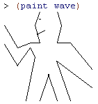
2.52a. Add some segments to the primitive wave painter of exercise 2.49 (to add a smile, for example).

This change requires that we make a change at a low level of abstraction, in adding segments to the wave painter itself. Let's add an eye and a smiling mouth on the left side of the head so it looks like the person in wave is looking in that direction.

; The wave painter (2.49d).
; Add some segments to form a smile (2.52a)
(define wave-segments
(list
(make-segment
(make-vect 0.006 0.840)
(make-vect 0.155 0.591))
(make-segment
(make-vect 0.006 0.635)
(make-vect 0.155 0.392))
(make-segment
(make-vect 0.304 0.646)
(make-vect 0.155 0.591))
(make-segment
(make-vect 0.298 0.591)
(make-vect 0.155 0.392))
(make-segment
(make-vect 0.304 0.646)
(make-vect 0.403 0.646))
(make-segment
(make-vect 0.298 0.591)
(make-vect 0.354 0.492))
(make-segment ; left face
(make-vect 0.403 0.646)
(make-vect 0.348 0.845))
(make-segment
(make-vect 0.354 0.492)
(make-vect 0.249 0.000))
(make-segment
(make-vect 0.403 0.000)
(make-vect 0.502 0.293))
(make-segment
(make-vect 0.502 0.293)
(make-vect 0.602 0.000))
(make-segment
(make-vect 0.348 0.845)
(make-vect 0.403 0.999))
(make-segment
(make-vect 0.602 0.999)
(make-vect 0.652 0.845))
(make-segment
(make-vect 0.652 0.845)
(make-vect 0.602 0.646))
(make-segment
(make-vect 0.602 0.646)
(make-vect 0.751 0.646))
(make-segment
(make-vect 0.751 0.646)
(make-vect 0.999 0.343))
(make-segment
(make-vect 0.751 0.000)
(make-vect 0.597 0.442))
(make-segment
(make-vect 0.597 0.442)
(make-vect 0.999 0.144))
(make-segment ; eye
(make-vect 0.395 0.916)
(make-vect 0.410 0.916))
(make-segment ; smile
(make-vect 0.376 0.746)
(make-vect 0.460 0.790))))


2.52b.
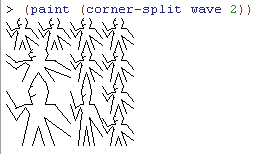
Change the pattern constructed by corner-split (for example, by using only one copy of the up-split and right-split images instead of two).

For this requirement we need to work in the middle layer of abstraction. To use only one copy of the up-split and right-split images instead of two, we can simply remove the references to top-left and bottom-right that appear in the original implementation of corner-split.

(define (corner-split painter n)
(if (= n 0)
painter
(let ((up (up-split painter (- n 1)))
(right (right-split painter (- n 1)))
(corner (corner-split painter (- n 1))))
(beside (below painter up)
(below right corner)))))


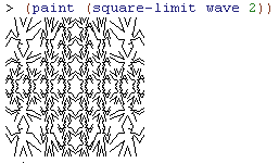
2.52c. Modify the version of square-limit that uses square-of-four so as to assemble the corners in a different pattern. (For example, you might make the big Mr. Rogers look outward from each corner of the square.)

We're not using the Mr. Rogers painter from the text, but we can still rearrange the square-limit painter so that the largest wave image is drawn in the four corners by simply rotating the corner-split painter by 180 degrees.

(define (square-limit painter n)
(let ((quarter (rotate180 (corner-split painter n))))
(let ((half (beside (flip-horiz quarter) quarter)))
(below (flip-vert half) half))))


Related:

For links to all of the SICP lecture notes and exercises that I've done so far, see The SICP Challenge.
Monday, January 2, 2012

SICP 2.50 - 2.51: Transforming and Combining Painters

From SICP section 2.2.4 Example: A Picture Language

Just as we did in exercises 2.44, 2.45, and 2.49, we can use the PLT Scheme SICP Picture Language package to run the solutions to the following exercises. You can load the picture package by putting the following (require...) expression at the beginning of your Scheme file.

(require (planet "sicp.ss" ("soegaard" "sicp.plt" 2 1)))

Exercise 2.50 asks us to define the transformation flip-horiz, which flips painters horizontally, and transformations that rotate painters counterclockwise by 180 degrees and 270 degrees.

We're expected to use the transform-painter procedure defined earlier in section 2.2.4 of the text. Since we're using the PLT Scheme SICP Picture Language package, we'll be using a version of transform-painter that's defined slightly differently than the one in the text. This procedure does not take the painter to be transformed as an argument, as does the version given in the text. Instead it takes the points that specify the corners of the new frame as arguments and returns a procedure that takes the painter as its argument.

For example, instead of defining flip-vert as:
(define (flip-vert painter)
(transform-painter painter
(make-vect 0.0 1.0) ; new origin
(make-vect 1.0 1.0) ; new end of edge1
(make-vect 0.0 0.0))) ; new end of edge2

We would instead pass the painter as an argument to the procedure returned from transform-painter as follows:
(define (flip-vertical painter)
((transform-painter (make-vect 0.0 1.0)
(make-vect 1.0 1.0)
(make-vect 0.0 0.0))
painter))

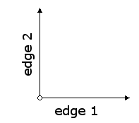
The arguments to transform-painter are points (represented as vectors) that specify the corners of the new frame. The first point specifies the new frame's origin and the other two specify the ends of its edge vectors. Remember that the origin point in a frame is normally in the lower left hand corner. The first edge vector is the bottom edge of frame and the second edge vector is the left edge of the frame.


These edges are defined by the points (0, 0) for the origin, (1, 0) for the end point of the first edge, and (0, 1) for the end point of the second edge. In order to transform a painter we just need to redraw the figure above in the desired orientation, then call transform-painter with the new positions of the origin and the end points of the edges.

To flip a painter horizontally we just move the origin and left edge to the right.


This gives the bottom edge a new endpoint as well. The procedure (based on flip-vert) would be:
(define (flip-horizontal painter)
((transform-painter (make-vect 1.0 0.0) ; origin
(make-vect 0.0 0.0) ; corner1
(make-vect 1.0 1.0)) ; corner2
painter))

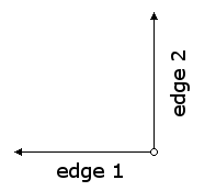
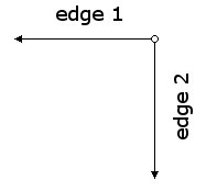
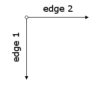
The following images show the locations of the origin and edges when we rotate an image counterclockwise by 180 and 270 degrees.


We can implement the procedures using the origin and endpoints shown in the figures above.
(define (rotate-180 painter)
((transform-painter (make-vect 1.0 1.0)
(make-vect 0.0 1.0)
(make-vect 1.0 0.0))
painter))

(define (rotate-270 painter)
((transform-painter (make-vect 0.0 1.0)
(make-vect 0.0 0.0)
(make-vect 1.0 1.0))
painter))

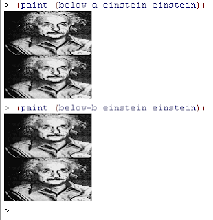
Use the einstein painter provided by the PLT Scheme SICP Picture Language package to check the output of the procedures above.


Exercise 2.51 asks us to define the below operation for painters. The below procedure takes two painters as arguments. The resulting painter draws the first painter in the bottom of the frame and the second painter in the top. We're asked to define below in two different ways -- first by writing a procedure that is analogous to the beside procedure given in the text, and again in terms of beside and suitable rotation operations like the ones we defined in exercise 2.50.

Translating the beside procedure from the text to create the first below procedure is a simple matter of applying what we learned in exercise 2.50 above.
(define (beside painter1 painter2)
(let ((split-point (make-vect 0.5 0.0)))
(let ((paint-left
(transform-painter painter1
(make-vect 0.0 0.0)
split-point
(make-vect 0.0 1.0)))
(paint-right
(transform-painter painter2
split-point
(make-vect 1.0 0.0)
(make-vect 0.5 1.0))))
(lambda (frame)
(paint-left frame)
(paint-right frame)))))

The beside procedure first defines a split-point at the bottom center of the frame that splits the frame vertically. It then transforms the two painters provided so that they each fit into one half of the frame. Finally, it returns a procedure that, when given a frame, paints the two images in the left and right halves of the frame. Here's the analogous below procedure:
; 2.51a
(define (below-a painter1 painter2)
(let ((split-point (make-vect 0.0 0.5)))
(let ((paint-bottom
((transform-painter (make-vect 0.0 0.0)
(make-vect 1.0 0.0)
split-point)
painter1))
(paint-top
((transform-painter split-point
(make-vect 1.0 0.5)
(make-vect 0.0 1.0))
painter2)))
(lambda (frame)
(paint-bottom frame)
(paint-top frame)))))

We need to redefine the split-point so that it divides the frame horizontally instead of vertically. We then transform the painters so that they fit into the bottom and top halves of the frame. Finally, we return a procedure that draws the two halves.

The second implementation of below is even simpler than the first. We just need to draw the two painters beside each other then rotate the frame by 90 degrees. When we do that the two images will be draw on their side, so we need to rotate the individual images 90 degrees in the opposite direction inside their smaller frames. This is equivalent to rotating them 270 degrees in the same direction.
; 2.51b
(define (rotate-90 painter)
((transform-painter (make-vect 1.0 0.0)
(make-vect 1.0 1.0)
(make-vect 0.0 0.0))
painter))

(define (below-b painter1 painter2)
(rotate-90 (beside (rotate-270 painter1) (rotate-270 painter2))))

Once again, we can test with einstein to verify that these two procedures both give us the desired output.


Related:

For links to all of the SICP lecture notes and exercises that I've done so far, see The SICP Challenge.
Sunday, October 9, 2011

SICP 2.49: Defining Primitive Painters

From SICP section 2.2.4 Example: A Picture Language

Exercise 2.49 asks us to use segments->painter to define the following primitive painters:

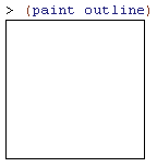
  1. The painter that draws the outline of the designated frame.
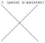
  2. The painter that draws an "X'' by connecting opposite corners of the frame.
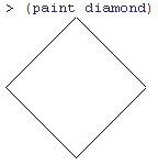
  3. The painter that draws a diamond shape by connecting the midpoints of the sides of the frame.
  4. The wave painter.

Just as we did in exercises 2.44 & 2.45, we can use the PLT Scheme SICP Picture Language package to run the exercises. You can load the picture package by putting the following (require...) expression at the beginning of your Scheme file.
(require (planet "sicp.ss" ("soegaard" "sicp.plt" 2 1)))

Since segments->painter takes a list of segments as its input parameter, each solution is just a matter of figuring out the coordinates of the endpoints of each required segment. Recall that the (0.0, 0.0) coordinate is the bottom left corner in the frame, not the top left corner as it is in many GUI environments. For each solution, we can define the list of segments first, then define a painter.
; 2.49 a.
; The painter that draws the outline of the designated frame.
(define outline-segments
(list
(make-segment
(make-vect 0.0 0.0)
(make-vect 0.0 0.99))
(make-segment
(make-vect 0.0 0.0)
(make-vect 0.99 0.0))
(make-segment
(make-vect 0.99 0.0)
(make-vect 0.99 0.99))
(make-segment
(make-vect 0.0 0.99)
(make-vect 0.99 0.99))))

(define outline (segments->painter outline-segments))

Note that I used 0.99 instead of 1.0 for the edges of the frame. This is because the top and right edges won't be displayed if you use 1.0.


; 2.49 b.
; The painter that draws an ``X'' by connecting opposite corners of the frame.
(define x-segments
(list
(make-segment
(make-vect 0.0 0.0)
(make-vect 0.99 0.99))
(make-segment
(make-vect 0.0 0.99)
(make-vect 0.99 0.0))))

(define x-painter (segments->painter x-segments))


; 2.49 c.
; The painter that draws a diamond shape by connecting the midpoints of the sides of the frame.
(define diamond-segments
(list
(make-segment
(make-vect 0.0 0.5)
(make-vect 0.5 0.0))
(make-segment
(make-vect 0.0 0.5)
(make-vect 0.5 0.999))
(make-segment
(make-vect 0.5 0.999)
(make-vect 0.999 0.5))
(make-segment
(make-vect 0.999 0.5)
(make-vect 0.5 0.0))))

(define diamond (segments->painter diamond-segments))


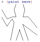
The wave painter in the last part of the exercise is the image shown in Figure 2.10 of the text. It consists of 17 separate segments.
; 2.49 d.
; The wave painter.
(define wave-segments
(list
(make-segment
(make-vect 0.006 0.840)
(make-vect 0.155 0.591))
(make-segment
(make-vect 0.006 0.635)
(make-vect 0.155 0.392))
(make-segment
(make-vect 0.304 0.646)
(make-vect 0.155 0.591))
(make-segment
(make-vect 0.298 0.591)
(make-vect 0.155 0.392))
(make-segment
(make-vect 0.304 0.646)
(make-vect 0.403 0.646))
(make-segment
(make-vect 0.298 0.591)
(make-vect 0.354 0.492))
(make-segment
(make-vect 0.403 0.646)
(make-vect 0.348 0.845))
(make-segment
(make-vect 0.354 0.492)
(make-vect 0.249 0.000))
(make-segment
(make-vect 0.403 0.000)
(make-vect 0.502 0.293))
(make-segment
(make-vect 0.502 0.293)
(make-vect 0.602 0.000))
(make-segment
(make-vect 0.348 0.845)
(make-vect 0.403 0.999))
(make-segment
(make-vect 0.602 0.999)
(make-vect 0.652 0.845))
(make-segment
(make-vect 0.652 0.845)
(make-vect 0.602 0.646))
(make-segment
(make-vect 0.602 0.646)
(make-vect 0.751 0.646))
(make-segment
(make-vect 0.751 0.646)
(make-vect 0.999 0.343))
(make-segment
(make-vect 0.751 0.000)
(make-vect 0.597 0.442))
(make-segment
(make-vect 0.597 0.442)
(make-vect 0.999 0.144))))

(define wave (segments->painter wave-segments))


Related:


For links to all of the SICP lecture notes and exercises that I've done so far, see The SICP Challenge.
Sunday, September 25, 2011

SICP 2.46 - 2.48: Frames & Painters

From SICP section 2.2.4 Example: A Picture Language

A frame can be described by three vectors -- an origin vector and two edge vectors. The origin vector specifies the offset of the frame's origin from some absolute origin in the plane, and the edge vectors specify the offsets of the frame's corners from its origin. If the edges are perpendicular, the frame will be rectangular. Otherwise the frame will be a more general parallelogram. A two-dimensional vector v running from the origin to a point can be represented as a pair consisting of an x-coordinate and a y-coordinate.

Exercise 2.46 asks us to implement a data abstraction for vectors by giving a constructor make-vect and corresponding selectors xcor-vect and ycor-vect. In terms of these selectors and constructor, we'll also implement procedures add-vect, sub-vect, and scale-vect that perform the operations for vector addition, vector subtraction, and multiplying a vector by a scalar:

(x1, y1) + (x2, y2) = (x1 + x2, y1 + y2)
(x1, y1) - (x2, y2) = (x1 - x2, y1 - y2)
s * (x, y) = (sx, sy)

The solution for the constructor and selectors uses cons, car, and cdr in the same pattern we've seen at least a dozen times by now.
(define (make-vect x y)
(cons x y))

(define (xcor-vect v)
(car v))

(define (ycor-vect v)
(cdr v))

Once we have those procedures in place, we can use them to build the vector operations specified.
(define (add-vect u v)
(make-vect
(+ (xcor-vect u) (xcor-vect v))
(+ (ycor-vect u) (ycor-vect v))))

(define (sub-vect u v)
(make-vect
(- (xcor-vect u) (xcor-vect v))
(- (ycor-vect u) (ycor-vect v))))

(define (scale-vect s v)
(make-vect
(* s (xcor-vect v))
(* s (ycor-vect v))))

We can test these procedures out with a few known values before moving on to the next step.
> (define u (make-vect 2 4))
> u
(2 . 4)
> (define v (make-vect 3 1))
> v
(3 . 1)
> (define w (add-vect u v))
> w
(5 . 5)
> (define x (sub-vect w u))
> x
(3 . 1)
> (define y (scale-vect 3 w))
> y
(15 . 15)


Exercise 2.47 gives us the following constructors for frames, one using list and the other using cons:
(define (make-frame origin edge1 edge2)
(list origin edge1 edge2))

(define (make-frame origin edge1 edge2)
(cons origin (cons edge1 edge2)))

We're asked to supply the appropriate selectors to produce an implementation for frames for each of the two constructors. Like any selector implementation, the task here is simply to extract each piece from the assembled object. We'll follow the naming convention from the previous exercise and call our selectors origin-frame, edge1-frame, and edge2-frame. Let's start with the version that uses list.
; 2.47a
(define (make-frame origin edge1 edge2)
(list origin edge1 edge2))

(define (origin-frame frame)
(car frame))

(define (edge1-frame frame)
(car (cdr frame)))

(define (edge2-frame frame)
(car (cdr (cdr frame))))

The selectors simply use the right combinations of car and cdr to extract the appropriate elements from the list. We can test it with some of the same values used in the previous exercise, but we'll need to add an origin vector.
> (define f (make-frame (make-vect 0 0) (make-vect 2 4) (make-vect 3 1)))
> f
((0 . 0) (2 . 4) (3 . 1))
> (origin-frame f)
(0 . 0)
> (edge1-frame f)
(2 . 4)
> (edge2-frame f)
(3 . 1)

Because the internal representation of a frame is different in the second implementation of make-frame, one of the selectors will have to change for the second part of the exercise. The original origin-frame and edge1-frame implementations will still work, but the edge2-frame procedure causes an error if you try to use it.
; 2.47b
(define (make-frame origin edge1 edge2)
(cons origin (cons edge1 edge2)))

(define (edge2-frame frame)
(cdr (cdr frame)))

Run exactly the same test from above to verify that you get the same results (except for the internal structure of the frame in the second step).
> (define f (make-frame (make-vect 0 0) (make-vect 2 4) (make-vect 3 1)))
> f
((0 . 0) (2 . 4) 3 . 1)
> (origin-frame f)
(0 . 0)
> (edge1-frame f)
(2 . 4)
> (edge2-frame f)
(3 . 1)


Exercise 2.48 asks us to define a representation for segments using our vector representation from exercise 2.46 above. We'll need to define the constructor make-segment and the selectors start-segment and end-segment.
(define (make-segment v1 v2)
(cons v1 v2))

(define (start-segment segment)
(car segment))

(define (end-segment segment)
(cdr segment))

Again, these use the same pattern we've seen before. In the next exercise, we'll take a closer look at the procedures above by drawing pictures with line segments using The SICP Picture Language package.


Related:

For links to all of the SICP lecture notes and exercises that I've done so far, see The SICP Challenge.
Saturday, August 20, 2011

SICP 2.44 & 2.45: A Picture Language

From SICP section 2.2.4 Example: A Picture Language

The next section of SICP is an extended example that illustrates the features of the picture language introduced in SICP Lecture 3A: Henderson Escher Example. I'm going to be using the PLT Scheme SICP Picture Language package to run the examples and exercises. You can load the picture package by putting the following (require...) expression at the beginning of your Scheme file.
(require (planet "sicp.ss" ("soegaard" "sicp.plt" 2 1)))


The painter primitive in the PLT package behaves slightly differently than the one presented in the text, in that it doesn't display itself. To display a painter you must call the paint procedure, which takes a painter as its argument.
> (paint einstein)


> (paint diagonal-shading)

The einstein and diagonal-shading painter values are built in to the PLT Scheme Picture Language package. The package also includes procedures for flipping, rotating and combining painter values, similar to those discussed in the lecture.
> (paint (flip-horiz einstein))


> (paint (flip-vert einstein))


> (paint (rotate90 einstein))


> (paint (beside einstein einstein))


> (paint (below einstein einstein))

Now that we can work with painters, we can start to combine them in ways that form patterns. For example, the text shows us how we can combine an image beside a flipped representation of itself, then draw the resulting painter below itself.
(define (flipped-pairs painter)

(let ((painter2 (beside painter (flip-vert painter))))
(below painter2 painter2)))

> (paint (flipped-pairs einstein))


We can also define recursive operations, like right-split, which makes painters split and branch towards the right as many times as we specify.
(define (right-split painter n)

(if (= n 0)
painter
(let ((smaller (right-split painter (- n 1))))
(beside painter (below smaller smaller)))))

> (paint (right-split einstein 3))


Exercise 2.44 asks us to define the procedure up-split. It's similar to right-split, except that it switches the roles of below and beside.
(define (up-split painter n)

(if (= n 0)
painter
(let ((smaller (up-split painter (- n 1))))
(below painter (beside smaller smaller)))))

> (paint (up-split einstein 3))


Once we have both right-split and up-split defined, we can create balanced patterns by branching in both directions.
(define (corner-split painter n)

(if (= n 0)
painter
(let ((up (up-split painter (- n 1)))
(right (right-split painter (- n 1))))
(let ((top-left (beside up up))
(bottom-right (below right right))
(corner (corner-split painter (- n 1))))
(beside (below painter top-left)
(below bottom-right corner))))))

> (paint (corner-split einstein 1))


> (paint (corner-split einstein 2))

By combining four copies of the corner-split pattern, we can create the square-limit pattern from the Escher drawing that we saw in the lecture.
(define (square-limit painter n)

(let ((quarter (corner-split painter n)))
(let ((half (beside (flip-horiz quarter) quarter)))
(below (flip-vert half) half))))

> (paint (square-limit einstein 4))


Exercise 2.45 points out that right-split and up-split can be expressed as instances of a general splitting operation. We are to define a split procedure, and then rewrite right-split and up-split in terms of split as follows:
(define right-split (split beside below))

(define up-split (split below beside))

We already noted the similarity between the two procedures right-split and up-split when we solved exercise 2.44 above. The only real difference between them is in which direction they split the painter first. Given the amount of duplication between the two, we can use either one of these procedures as a template for split.
(define (split dir1 dir2)

(lambda (painter n)
(if (= n 0)
painter
(let ((smaller ((split dir1 dir2) painter (- n 1))))
(dir1 painter (dir2 smaller smaller))))))

The biggest change is that split uses a lambda to return the procedure that it creates. Once you're done substituting the new definitions for right-split and up-split, you can run the square-limit procedure again to verify that the output hasn't changed.


Related:

For links to all of the SICP lecture notes and exercises that I've done so far, see The SICP Challenge.
Sunday, July 24, 2011

SICP Lecture 3A: Henderson Escher Example

Structure and Interpretation of Computer Programs
Henderson Escher Example
Covers Text Section 2.2.2

You can download the video lecture or stream it on MIT's OpenCourseWare site. It's also available on YouTube.

This lecture is presented by Professor Harold Abelson.

This lecture starts out with a review of the material covered in the previous lecture on compound data. The main points covered are pairs and the closure property (the things we make by forming pairs can also be combined to form pairs).

We're then shown how cons can be used to create lists of primitive elements in Scheme.
(cons 1
(cons 2
(cons 3
(cons 4 nil))))

is the same as
(list 1 2 3 4)

A common pattern in programming is to write procedures that takes a list, do something to every element of that list, and return a list containing the results. We saw an example, scale-list, that takes a list and a factor and returns the result of each element in the list multiplied by the factor.
(define (scale-list items factor)
(if (null? items)
nil
(cons (* (car items) factor)
(scale-list (cdr items) factor))))

In Scheme terms, the general pattern here is to recursively do something to the cdr of the list and cons that on to actually doing something to the first element of the list.
The very fact that there's a general pattern there means I shouldn't be writing this procedure at all.

Instead of embedding a general pattern in each procedure that uses it, we should write a procedure that's the general pattern itself and write our procedure in terms of that higher-order procedure. For this example, that higher-order procedure is map. (See SICP 2.21 - 2.23: Mapping over lists for examples.)
(define (map proc items)
(if (null? items)
nil
(cons (proc (car items))
(map proc (cdr items)))))

The important idea here is that we stop thinking about control structures and start thinking about applying operations to aggregates.


Henderson Escher Example

The remainder of the lecture talks about one particular example, the Henderson Escher Example, that summarizes everything that's been covered in the course so far, list structure, abstraction, representation, and capturing commonality with higher-order procedures. It also goes into the third major theme of the course, meta-linguistic abstraction.

Meta-linguistic abstraction:
  • Primitives
  • Means of Combination
  • Means of Abstraction

The example is a language developed by Peter Henderson for describing images that are composed of repeated elements that are shifted and scaled, like the M. C. Escher woodcut "Square Limit" pictured below.


The other theme illustrated by this example is the issue that there is no real difference between procedures and data.

The language operates on primitives called pictures. A picture is a procedure that draws a figure scaled to fit a rectangle that you specify. The following operations are supported in the language.

  • rotate - Rotate a picture 90 degrees.
  • flip - Flip a picture horizonally or vertically.
  • beside - Draw two pictures beside one another.
  • above - Draw two pictures, one above the other.

The closure property allows you to build complex pictures with just these few operations and one primitive (the picture itself). When you combine two pictures with beside or above, the result is itself a picture, which can be combined with other pictures.

We're going to see a lot of details concerning the implementation of the picture language illustrated in this example as we go through the exercises in the next section of the text, so I won't reproduce those details here. The gist is that we define one set of procedures to draw pictures inside of rectangles, another set of procedures that do the geometric manipulations of those pictures listed above (rotate, flip, beside, and above), then a higher-order set of procedures that combine those manipulated pictures in different ways to make an image like the Escher drawing above..


Software Design Methodologies

The last part of the lecture talks about the common software design methodology of decomposing a problem into discrete components, which are themselves decomposed into discrete components, and so on until you reach a design that looks like the tree structure below.


Each component in this kind of design is created to do one specific task, and the components only communicate with direct parent or child components in the hierarchy. Contrast this with the way the picture language was developed in the Henderson Escher example. First, a language for drawing primitive pictures was presented, then on top of that we build a language for geometric rotations, and finally, on top of that we built a language for schemes of combination.


This scheme gives you a full range of linguistic power at each level.

Lisp is a lousy language for doing any particular problem. What it's good for is figuring out the right language that you want and embedding that in Lisp.

For links to all of the SICP lecture notes and exercises that I've done so far, see The SICP Challenge.